Hamiltonian objects and reference frames#
For the examples below the following imports have already been executed:
>>> import astropy.units as u
>>> import numpy as np
>>> import matplotlib.pyplot as plt
>>> import gala.potential as gp
>>> import gala.dynamics as gd
>>> import gala.integrate as gi
>>> from gala.units import galactic
Introduction#
When integrating orbits using the potential classes directly, for example:
>>> pot = gp.HernquistPotential(m=1E10*u.Msun, c=1.*u.kpc,
...                             units=galactic)
>>> w0 = gd.PhaseSpacePosition(pos=[5.,0,0]*u.kpc,
...                            vel=[0,0,50.]*u.km/u.s)
>>> orbit = gp.Hamiltonian(pot).integrate_orbit(w0, dt=0.5, n_steps=1000)
it is implicitly assumed that the initial conditions and orbit are in an inertial (static) reference frame. In this case, the total energy or value of the Hamiltonian (per unit mass) is simply
It is sometimes useful to transform to alternate, non-inertial reference frames to do the numerical orbit integration. In this case, the _effective_ Hamiltonian may include other terms. For example, in the case of a rotating reference frame constantly rotating with frequency vector \(\boldsymbol{\Omega}\), the effective potential can be written
where \(\boldsymbol{L}\) is the angular momentum. For working in
non-inertial reference frames, Gala provides a way to compose potential objects
(which define just the static component of the effective potential) with
reference frame objects into a Hamiltonian
object, which can then be used for orbit integration, evaluating the full
symplectic gradient of the effective Hamiltonian, and computing the value
(pseudo-energy) of the effective Hamiltonian.
Creating a Hamiltonian object with a specified reference frame#
Using the potential objects and
integrate_orbit() to integrate
an orbit is equivalent to defining a
Hamiltonian object with the potential
object and a Staticframe instance:
>>> pot = gp.HernquistPotential(m=1E10*u.Msun, c=1.*u.kpc,
...                             units=galactic)
>>> frame = gp.StaticFrame(units=galactic)
>>> H = gp.Hamiltonian(potential=pot, frame=frame)
>>> w0 = gd.PhaseSpacePosition(pos=[5.,0,0]*u.kpc,
...                            vel=[0,0,50.]*u.km/u.s)
>>> orbit = H.integrate_orbit(w0, dt=0.5, n_steps=1000)
In this case, the orbit object returned from integration knows what
reference frame it is in and we can therefore transform it to other reference
frames. For example, we can change to a constantly rotating frame with a
frequency vector that determines the axis of rotation and angular velocity of
rotation around that axis:
>>> rotation_axis = np.array([8.2, -1.44, 3.25])
>>> rotation_axis /= np.linalg.norm(rotation_axis) # make a unit vector
>>> frame_freq = 42. * u.km/u.s/u.kpc
>>> rot_frame = gp.ConstantRotatingFrame(Omega=frame_freq * rotation_axis,
... units=galactic)
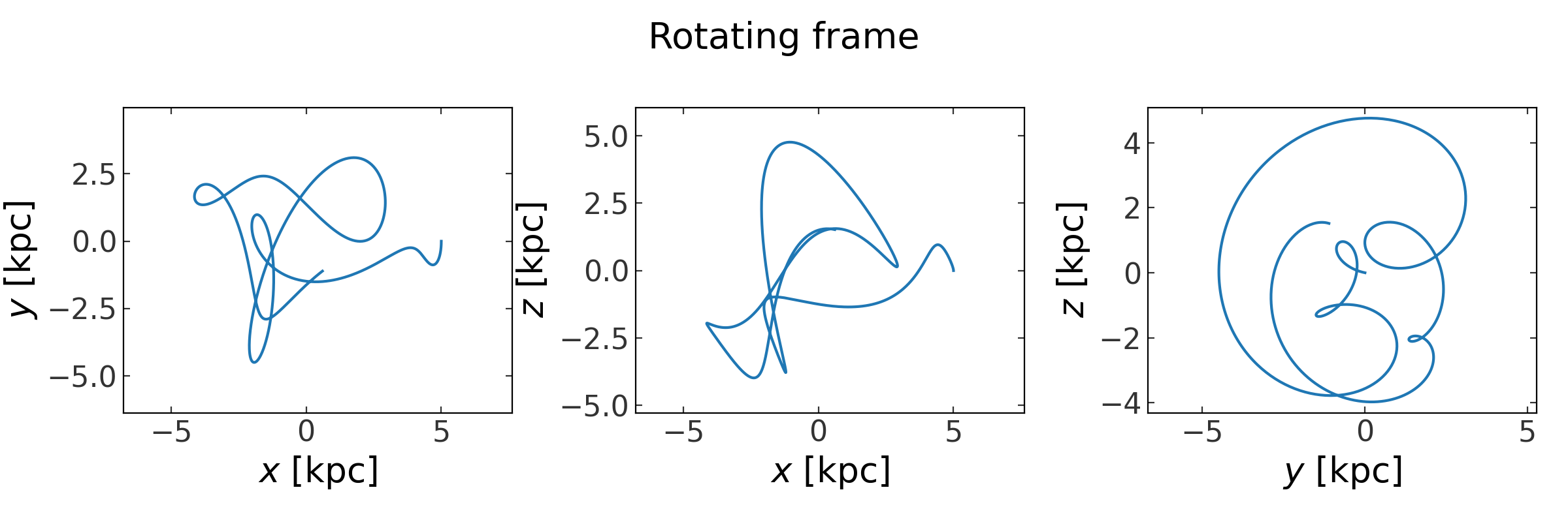
>>> orbit_to_rot = orbit.to_frame(rot_frame)
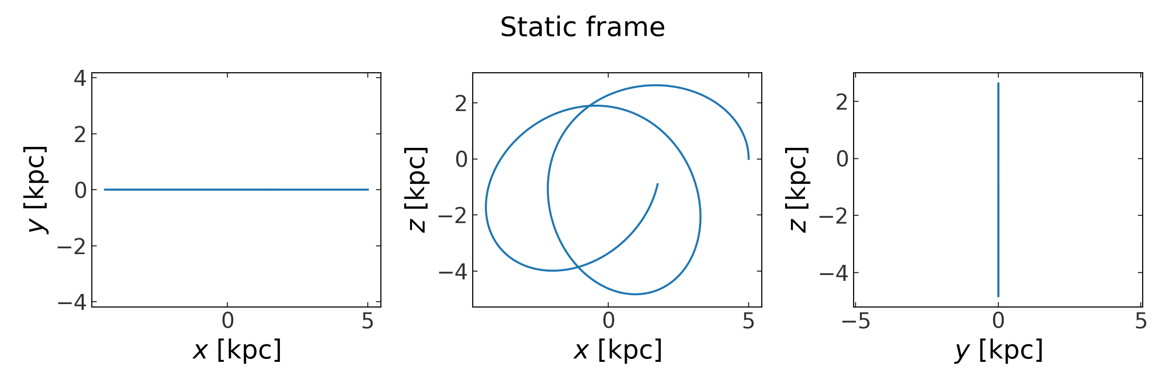
>>> fig1 = orbit.plot(marker='')
>>> fig1.suptitle("Static frame")
>>> fig2 = rot_orbit.plot(marker='')
>>> fig2.suptitle("Rotating frame")
We can also integrate the orbit in the rotating frame directly by creating a
Hamiltonian object with the rotating
frame:
>>> H_rot = gp.Hamiltonian(potential=pot, frame=rot_frame)
>>> rot_orbit = H_rot.integrate_orbit(w0, dt=0.5, n_steps=1000)
>>> _ = rot_orbit.plot(marker='')
(Source code, png, pdf)
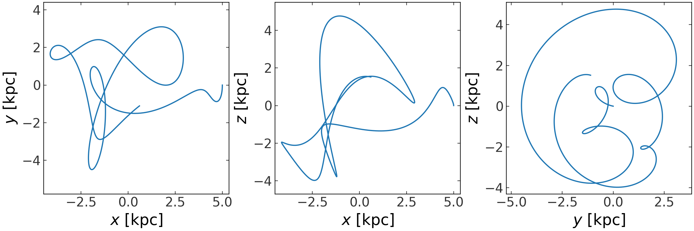
In this case, because the potential is spherical, the orbit should look the same whether we integrate it in the rotating frame or in a static frame and then transform to a rotating frame. In the example below, we consider the case of integrating orbits in an asymmetric, time-dependent bar potential.
See the integrate_rotating_frame example for more information.