Integrating and plotting an orbit in an NFW potential

We first import the required packages:

>>> import astropy.units as u
>>> import matplotlib.pyplot as plt
>>> import numpy as np
>>> import gala.integrate as gi
>>> import gala.dynamics as gd
>>> import gala.potential as gp
>>> from gala.units import galactic

In the examples below, we’ll use the galactic UnitSystem: kpc, Myr, \({\rm M}_\odot\), radians.

We’ll create an NFW potential parametrized by a scale radius and circular velocity at the scale radius:

>>> pot = gp.NFWPotential.from_circular_velocity(v_c=200*u.km/u.s,
...                                              r_s=10.*u.kpc,
...                                              units=galactic)

Now we’ll integrate a single orbit in this potential. The easiest approach is to use the integrate_orbit method, which accepts initial conditions and time-stepping specification. We define the initial conditions as a PhaseSpacePosition object:

>>> ics = gd.PhaseSpacePosition(pos=[10,0,0.] * u.kpc,
...                             vel=[0,175,0] * u.km/u.s)
>>> orbit = gp.Hamiltonian(pot).integrate_orbit(ics, dt=2., n_steps=2000)

This returns a Orbit object containing times and 6D positions at each time step. By default, this uses Leapfrog integration (LeapfrogIntegrator), but you can specify a different integrator by passing the integrator class:

>>> orbit = gp.Hamiltonian(pot).integrate_orbit(ics, dt=2., n_steps=2000,
...                             Integrator=gi.DOPRI853Integrator)

or more conveniently, by passing a string name:

>>> orbit = gp.Hamiltonian(pot).integrate_orbit(ics, dt=2., n_steps=2000,
...                             Integrator='dopri853')

We can integrate many orbits in parallel by passing a 2D array of initial conditions. Here, we’ll generate random initial conditions by sampling from a Gaussian around the initial orbit (positional scale: 100 pc, velocity scale: 1 km/s):

>>> norbits = 128
>>> new_pos = np.random.normal(ics.pos.xyz.to(u.pc).value, 100.,
...                            size=(norbits,3)).T * u.pc
>>> new_vel = np.random.normal(ics.vel.d_xyz.to(u.km/u.s).value, 1.,
...                            size=(norbits,3)).T * u.km/u.s
>>> new_ics = gd.PhaseSpacePosition(pos=new_pos, vel=new_vel)
>>> orbits = gp.Hamiltonian(pot).integrate_orbit(new_ics, dt=2., n_steps=2000)

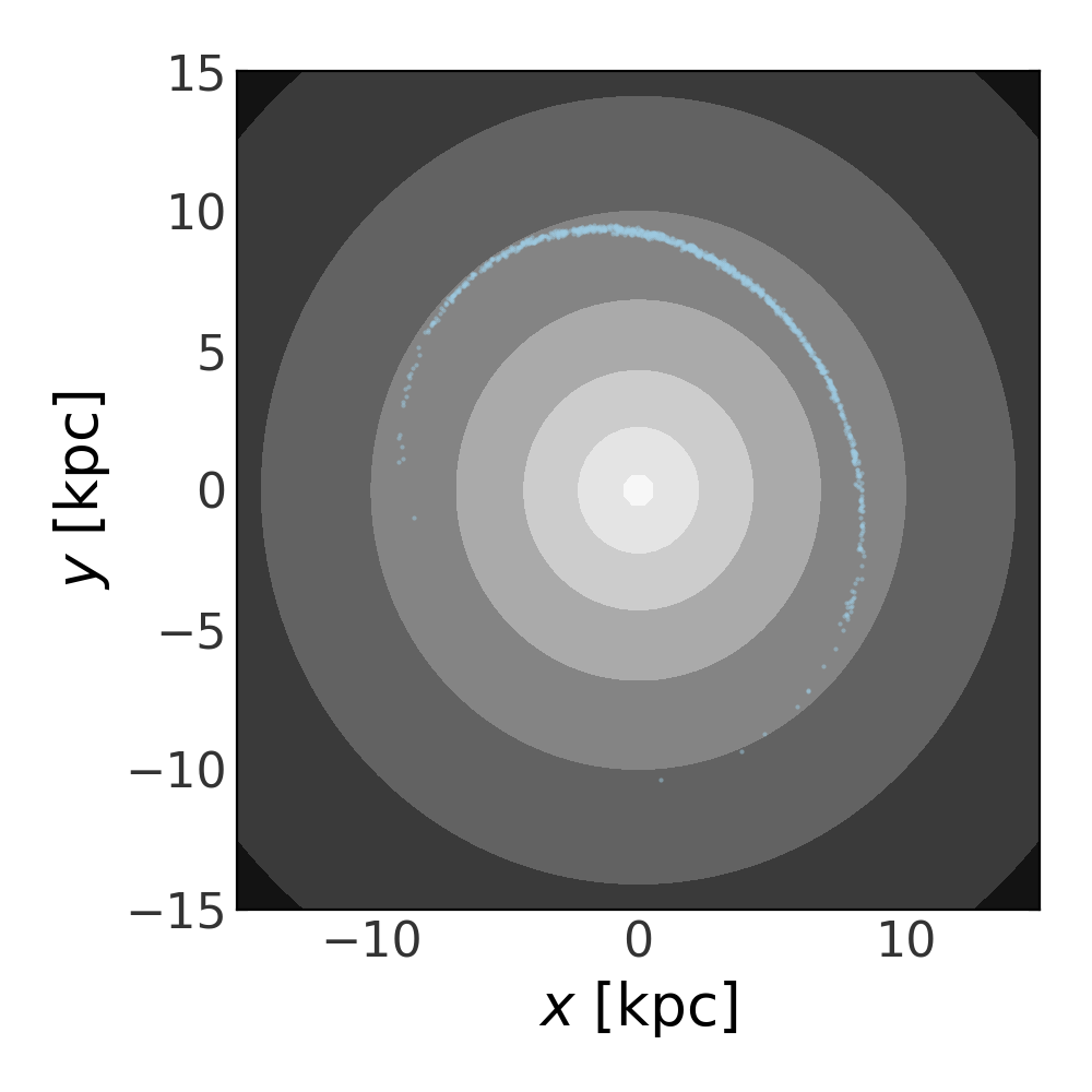
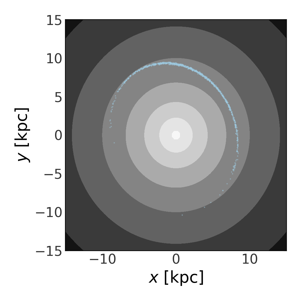
Now we’ll plot the final positions of these orbits over isopotential contours. We use the plot_contours() method to plot potential contours, then overplot the orbit points:

>>> grid = np.linspace(-15,15,64)
>>> fig,ax = plt.subplots(1, 1, figsize=(5,5))
>>> fig = pot.plot_contours(grid=(grid,grid,0), cmap='Greys', ax=ax)
>>> fig = orbits[-1].plot(['x', 'y'], color='#9ecae1', s=1., alpha=0.5,
...                       axes=[ax], auto_aspect=False)

(Source code, png, pdf)