Getting Started#
Welcome to the gala documentation!
For practical reasons, this documentation generally assumes that you are
familiar with the Python programming language, including numerical and
computational libraries like numpy, scipy, and matplotlib. If you need a refresher on Python programming, we
recommend starting with the official Python tutorial, but many other good resources are
available on the internet, such as tutorials and lectures specifically designed
for using Python for scientific applications.
On this introductory page, we will demonstrate a few common use cases for gala
and give an overview of the package functionality. For the examples
below, we will assume that the following imports have already been executed
because these packages will be generally required:
>>> import astropy.units as u
>>> import numpy as np
Computing your first stellar orbit#
One of the most common use cases for gala is computing stellar orbits within
a Milky Way mass model. This requires two things: (1) a gravitational potential
model representing the Milky Way’s mass distribution, and (2) initial conditions
for the star’s orbit.
Mass models in gala are specified using Python classes that represent
gravitational potential models. The standard Milky Way model recommended for
use in gala is the MilkyWayPotential version=”latest”,
which is a pre-defined, multi-component model of the Milky Way with parameters set to
match the rotation curve of the Galactic disk and the mass profile of the dark matter
halo:
>>> import gala.potential as gp
>>> mw = gp.MilkyWayPotential(version="latest")
>>> mw
<CompositePotential disk,bulge,nucleus,halo>
This model contains four distinct potential components: disk, bulge, nucleus,
and halo. You can configure any of these component parameters or create custom
composite potential models (see gala.potential), but for now we’ll use the
default model.
All potential classes in gala.potential have standard methods for computing
dynamical quantities. For example, we can compute the potential energy and acceleration
at a Cartesian position near the Sun:
>>> xyz = [-8.0, 0.0, 0.0] * u.kpc
>>> mw.energy(xyz)
<Quantity [-0.16440296] kpc2 / Myr2>
>>> mw.acceleration(xyz)
<Quantity [[ 0.00702262],
           [-0.        ],
           [-0.        ]] kpc / Myr2>
The returned values are Astropy Quantity objects with
associated physical units. These can be converted to any equivalent units:
>>> E = mw.energy(xyz)
>>> E.to((u.km / u.s) ** 2)
<Quantity [-157181.98979398] km2 / s2>
>>> acc = mw.acceleration(xyz)
>>> acc.to(u.km / u.s / u.Myr)
<Quantity [[ 6.86666358],
           [-0.        ],
           [-0.        ]] km / (Myr s)>
Now to compute an orbit, we need initial conditions. In gala, phase-space
positions are defined using the PhaseSpacePosition class.
As an example, we’ll use initial conditions close to the Sun’s Galactocentric
position and velocity:
>>> import gala.dynamics as gd
>>> w0 = gd.PhaseSpacePosition(
...     pos=[-8.1, 0, 0.02] * u.kpc,
...     vel=[13, 245, 8.0] * u.km / u.s,
... )
I use the variable w to represent phase-space positions, so w0
represents initial conditions. When passing Cartesian position and velocity
values, they must be Quantity objects with units whenever
the potential has a dimensional unit system:
>>> mw.units
<UnitSystem (kpc, Myr, solMass, rad)>
Our Milky Way potential uses dimensional units. You can use any compatible
length and velocity units, as gala handles unit conversions internally.
With a potential model and initial conditions defined, we can now compute an
orbit using the integrate_orbit()
method:
>>> orbit = mw.integrate_orbit(w0, dt=1 * u.Myr, t1=0, t2=2 * u.Gyr)
This uses Leapfrog integration by default, which is a fast, symplectic
integration scheme. The returned Orbit object represents
a collection of phase-space positions at different times:
>>> orbit
<Orbit cartesian, dim=3, shape=(2000,)>
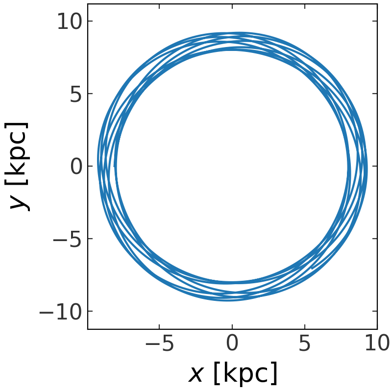
Orbit objects have many of their own useful methods for
performing common tasks, like plotting an orbit:
>>> orbit.plot(["x", "y"])
(Source code, png, pdf)

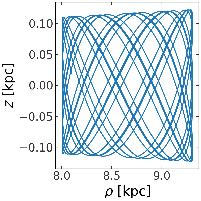
Orbit objects by default assume and use Cartesian coordinate
representations, but these can also be transformed into other representations,
like Cylindrical coordinates. For example, we could re-represent the orbit in
cylindrical coordinates and then plot the orbit in the “meridional plane”:
>>> fig = orbit.cylindrical.plot(["rho", "z"])
(Source code, png, pdf)
Or estimate the pericenter, apocenter, and eccentricity of the orbit:
>>> orbit.pericenter()
<Quantity 8.00498069 kpc>
>>> orbit.apocenter()
<Quantity 9.30721946 kpc>
>>> orbit.eccentricity()
<Quantity 0.07522087>
gala.potential Potential objects and Orbit objects have
many more possibilities, so please do check out the narrative documentation for
gala.potential and gala.dynamics if you would like to learn more!
What else can gala do?#
This page is meant to demonstrate a few initial things you may want to do with
gala. There is much more functionality that you can discover either through
the tutorials or by perusing the user guide. Some other commonly-used functionality includes:
Where to go from here#
The two places to learn more are the tutorials and the user guide:
The Tutorials are narrative demonstrations of functionality that walk through simplified, real-world use cases for the tools available in
gala.The User Guide contains more exhaustive descriptions of all of the functions and classes available in
gala, and should be treated more like reference material.