
Gravitational potentials (gala.potential)#
Introduction#
This subpackage provides a number of classes for working with parametric models
of gravitational potentials. There are a number of built-in potentials
implemented in C and Cython (for speed), and there are base classes that allow
for easy creation of new custom potential classes
in pure Python or by writing custom C/Cython extensions. The Potential
objects have convenience methods for computing common dynamical quantities, for
example: potential energy, spatial gradient, density, or mass profiles. These
are particularly useful in combination with the integrate and
dynamics subpackages.
Also defined in this subpackage are a set of reference frames which can be used
for numerical integration of orbits in non-static reference frames. See the page
on Hamiltonian objects and reference frames for more information. Potential
objects can be combined with a reference frame and stored in a
Hamiltonian object that provides an easy interface
to numerical orbit integration.
For the examples below the following imports have already been executed:
>>> import astropy.units as u
>>> import matplotlib.pyplot as plt
>>> import numpy as np
>>> import gala.potential as gp
>>> from gala.units import galactic, solarsystem, dimensionless
Getting Started: Built-in Methods of Potential Classes#
Potential classes are initialized by passing parameter values as
Quantity objects or as numeric values with a
specified unit system. You must also specify a UnitSystem
— a set of non-reducible units defining length, mass, time, and angle units.
Common unit systems are built in (e.g., galactic, solarsystem,
dimensionless).
For example, to create a Kepler potential (point mass) with mass = 1 solar mass:
>>> ptmass = gp.KeplerPotential(m=1.0 * u.Msun, units=solarsystem)
>>> ptmass
<KeplerPotential: m=1.00 (AU,yr,solMass,rad)>
Parameters with different units are automatically converted to the specified unit system:
>>> gp.KeplerPotential(m=1047.6115 * u.Mjup, units=solarsystem)
<KeplerPotential: m=1.00 (AU,yr,solMass,rad)>
Parameters without units are assumed to be in the specified unit system:
>>> gp.KeplerPotential(m=1.0, units=solarsystem)
<KeplerPotential: m=1.00 (AU,yr,solMass,rad)>
To work without units, use DimensionlessUnitSystem or pass
None (this is the default, so you can also omit the units argument):
>>> gp.KeplerPotential(m=1.0, units=None)
<KeplerPotential: m=1.00 (dimensionless)>
Unit systems can also be specified by passing a string name:
>>> gp.KeplerPotential(m=1.0 * u.Msun, units='solarsystem')
<KeplerPotential: m=1.00 (AU,yr,solMass,rad)>
All built-in potential objects have methods to evaluate the potential energy
and gradient/acceleration at given positions. For example, to evaluate the
potential energy at (x, y, z) = (1, -1, 0) AU:
>>> ptmass.energy([1.0, -1.0, 0.0] * u.au)
<Quantity [-27.91440236] AU2 / yr2>
These functions accept both Quantity objects and
plain array-like objects (assumed to be in the potential’s unit system):
>>> ptmass.energy([1.0, -1.0, 0.0])
<Quantity [-27.91440236] AU2 / yr2>
For multiple positions, pass a 2D array where each column is a position:
>>> pos = np.array([[1.0, -1.0, 0], [2.0, 3.0, 0]]).T
>>> ptmass.energy(pos * u.au)
<Quantity [-27.91440236, -10.94892941] AU2 / yr2>
We can also compute the gradient or acceleration:
>>> ptmass.gradient([1.0, -1.0, 0] * u.au)
<Quantity [[ 13.95720118],
           [-13.95720118],
           [  0.        ]] AU / yr2>
>>> ptmass.acceleration([1.0, -1.0, 0] * u.au)
<Quantity [[-13.95720118],
           [ 13.95720118],
           [ -0.        ]] AU / yr2>
Using Symmetry Coordinates#
Many potentials have symmetries that make certain coordinate systems more natural or concise to work with. For example, spherically-symmetric potentials only depend on the radius \(r\), and axisymmetric potentials only depend on the cylindrical radius \(R\) and height \(z\).
For potentials with these symmetries, you can use symmetry coordinates as a shorthand instead of full 3D Cartesian coordinates. Internally, gala operates in Cartesian coordinates, so the symmetry coordinates are simply a front-end convenience.
Spherical Potentials#
For spherically-symmetric potentials (like HernquistPotential,
PlummerPotential, KeplerPotential,
etc.), you can pass just the radius using r=:
>>> pot = gp.HernquistPotential(m=1e10 * u.Msun, c=5 * u.kpc, units=galactic)
>>> r = np.array([1.0, 5.0, 10.0]) * u.kpc
>>> pot.energy(r=r)
<Quantity [-0.06674208, -0.03367003, -0.01792115] kpc2 / Myr2>
This is equivalent to passing Cartesian coordinates [r, 0, 0], but much cleaner. All
potential methods support symmetry coordinates:
>>> pot.gradient(r=r)  # Note: Still returns gradient in Cartesian
>>> pot.density(r=r)
>>> pot.mass_enclosed(r=r)
>>> pot.circular_velocity(r=r)
Note that gradients and accelerations are always returned in Cartesian coordinates, even when using symmetry inputs. This ensures consistency and compatibility with orbit integration.
Cylindrical (Axisymmetric) Potentials#
For axisymmetric potentials (like MiyamotoNagaiPotential),
you can use cylindrical coordinates with R= and z=:
>>> pot = gp.MiyamotoNagaiPotential(m=1e11 * u.Msun, a=3 * u.kpc, b=0.3 * u.kpc, units=galactic)
>>> R = np.linspace(4, 12, 100) * u.kpc
>>> z = np.linspace(-1, 1, 100) * u.kpc
>>> pot.energy(R=R, z=z)
The z coordinate defaults to zero, making midplane calculations particularly
convenient:
>>> pot.energy(R=R) # Evaluate in the midplane (z=0)
This is especially useful for plotting rotation curves or computing circular velocities in the disk plane.
Most of the potential objects also have methods implemented for computing the
corresponding mass density and the Hessian of the potential (the matrix of 2nd
derivatives) at given locations. For example, with the
HernquistPotential, we can evaluate both the
mass density and Hessian at the position (x, y, z) = (1, -1, 0) kpc:
>>> pot = gp.HernquistPotential(m=1e9 * u.Msun, c=1.0 * u.kpc, units=galactic)
>>> pot.density([1.0, -1.0, 0] * u.kpc)
<Quantity [7997938.82200887] solMass / kpc3>
>>> pot.hessian([1.0, -1.0, 0] * u.kpc)
<Quantity [[[ -4.68318131e-05],
            [  5.92743432e-04],
            [  0.00000000e+00]],

           [[  5.92743432e-04],
            [ -4.68318131e-05],
            [  0.00000000e+00]],

           [[  0.00000000e+00],
            [  0.00000000e+00],
            [  5.45911619e-04]]] 1 / Myr2>
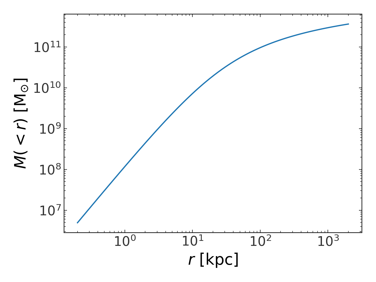
Another useful method is
mass_enclosed(), which numerically
estimates the mass enclosed within a spherical shell defined by the specified
position. This numerically estimates \(\frac{d \Phi}{d r}\) along the vector
pointing at the specified position and estimates the enclosed mass simply as
\(M(<r)\approx\frac{r^2}{G} \frac{d \Phi}{d r}\). This function can be used
to compute, for example, a mass profile. For spherical potentials, you can use
the r= symmetry coordinate:
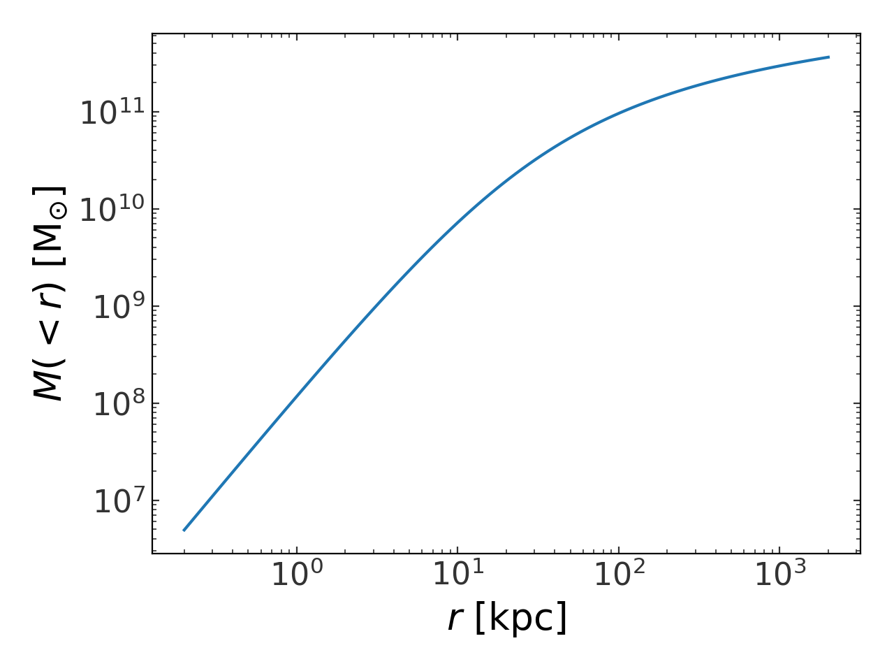
>>> pot = gp.NFWPotential(m=1e11 * u.Msun, r_s=20.0 * u.kpc, units=galactic)
>>> r = np.logspace(np.log10(20.0 / 100.0), np.log10(20 * 100.0), 100) * u.kpc
>>> m_profile = pot.mass_enclosed(r=r)
>>> plt.loglog(r, m_profile, marker="")
>>> plt.xlabel("$r$ [{}]".format(r.unit.to_string(format="latex")))
>>> plt.ylabel("$M(<r)$ [{}]".format(m_profile.unit.to_string(format="latex")))
(Source code, png, pdf)
Plotting Equipotential and Isodensity contours#
Potential objects provide methods for visualizing isopotential
(plot_contours()) and isodensity
(plot_density_contours()) contours.
These methods create either 1D slices or 2D contour plots.
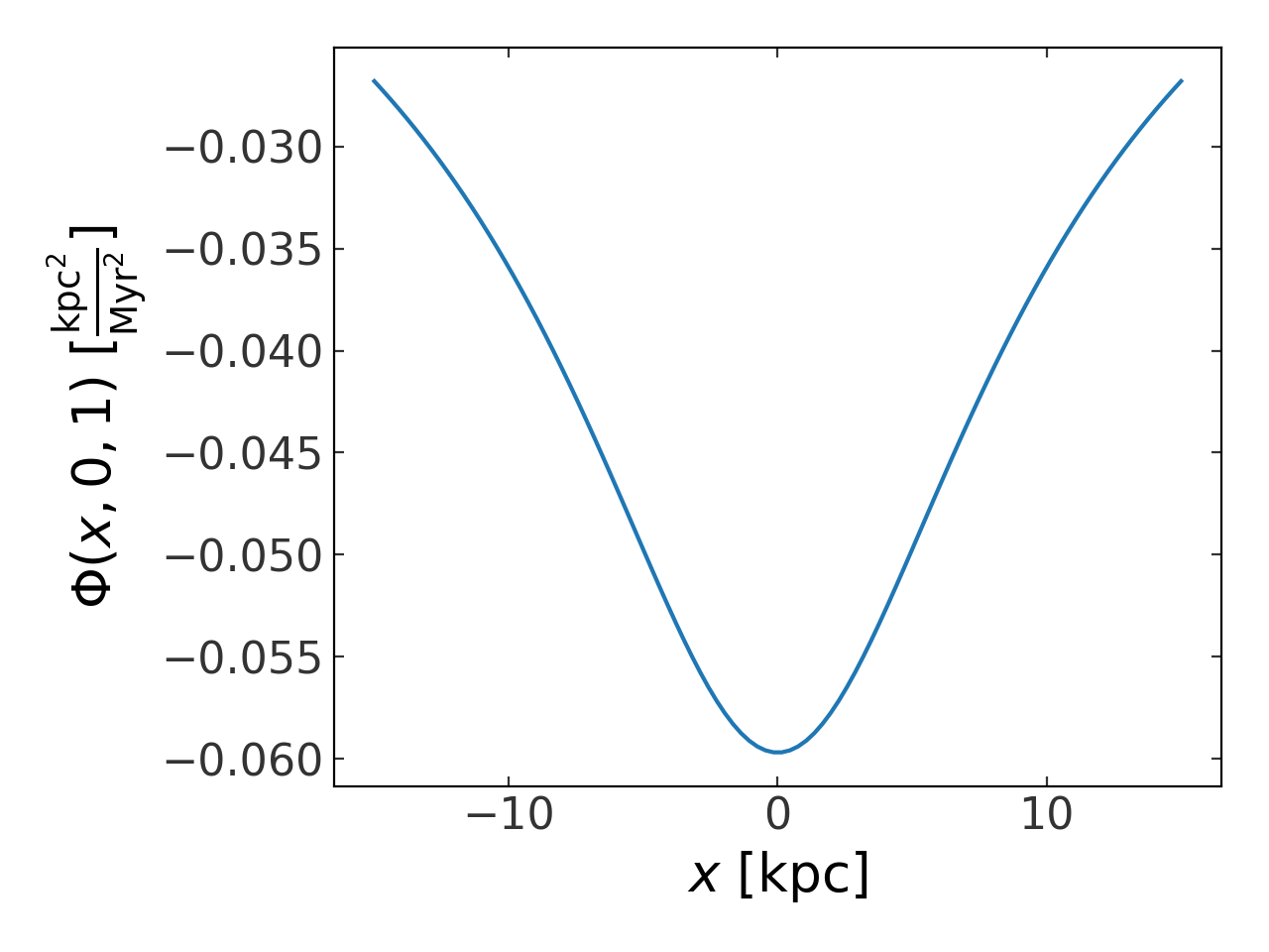
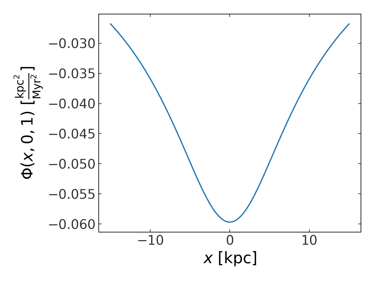
For a 1D slice, pass a grid for one dimension and fixed values for others. For example, to plot potential vs. \(x\) at \(y=0, z=1\):
>>> p = gp.MiyamotoNagaiPotential(m=1e11, a=6.5, b=0.27, units=galactic)
>>> fig, ax = plt.subplots()
>>> p.plot_contours(
...     grid=(np.linspace(-15, 15, 100), 0.0, 1.0), marker="", ax=ax
... )
(Source code, png, pdf)
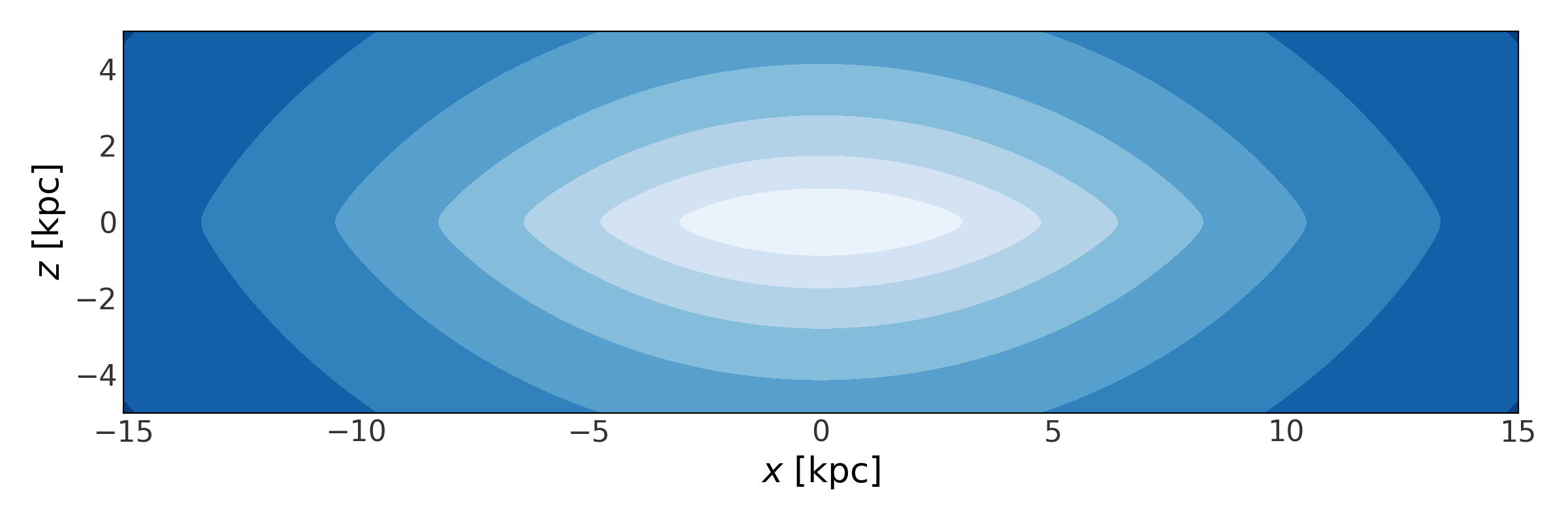
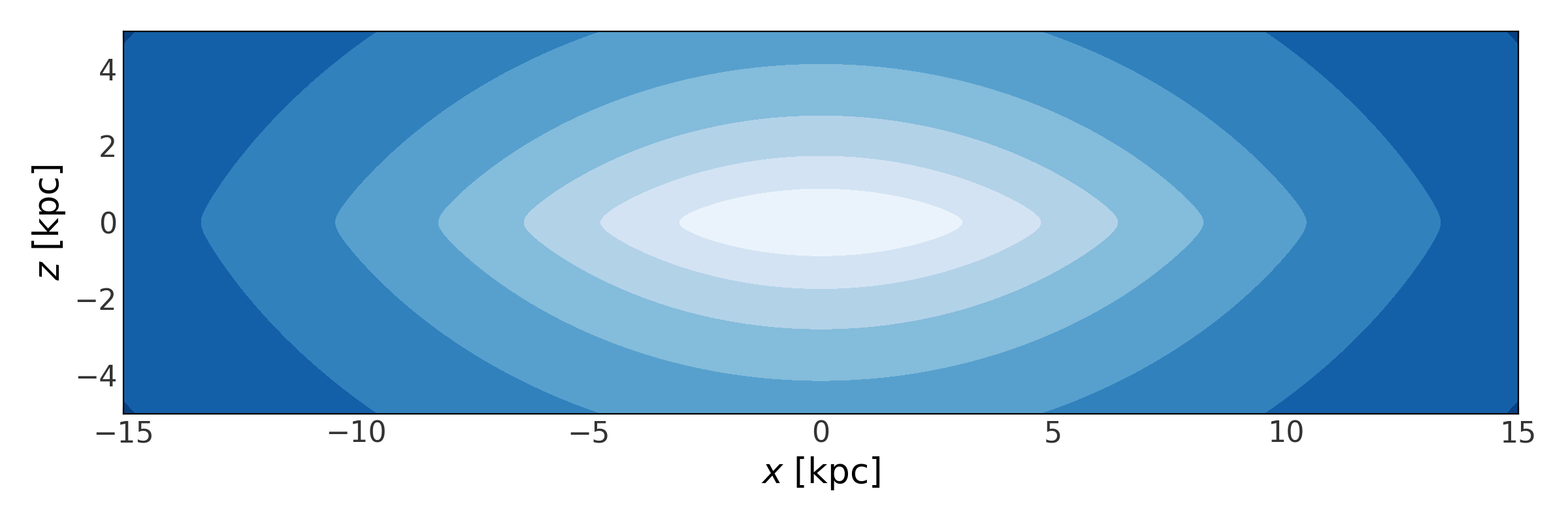
For 2D contour plots, pass 1D grids for two dimensions and a fixed value for the third. For example, to plot \(x\)-\(z\) contours at \(y=0\):
>>> fig, ax = plt.subplots(1, 1, figsize=(12, 4))
>>> x = np.linspace(-15, 15, 100)
>>> z = np.linspace(-5, 5, 100)
>>> p.plot_contours(grid=(x, 1.0, z), ax=ax)
(Source code, png, pdf)
Saving / loading potential objects#
Potential objects can be saved to and loaded from YAML files using the
save() method and
load() function:
>>> from gala.potential import load
>>> pot = gp.NFWPotential(m=6e11 * u.Msun, r_s=20.0 * u.kpc, units=galactic)
>>> pot.save("potential.yml")
>>> load("potential.yml")
<NFWPotential: m=6.00e+11, r_s=20.00, a=1.00, b=1.00, c=1.00 (kpc,Myr,solMass,rad)>
Exporting potentials as sympy expressions#
Most of the potential classes can be exported to a sympy expression that can
be used to manipulate or evaluate the form of the potential. To access this
functionality, the potential classes have a
to_sympy classmethod (note: this
requires sympy to be installed):
>>> expr, vars_, pars = gp.LogarithmicPotential.to_sympy()
>>> str(expr)
'0.5*v_c**2*log(r_h**2 + z**2/q3**2 + y**2/q2**2 + x**2/q1**2)'
This method also returns a dictionary containing the coordinate variables used
in the expression as sympy symbols, here defined as vars_:
>>> vars_
{"x": x, "y": y, "z": z}
A second dictionary containing the potential parameters as sympy symbols is
also returned, here defined as pars:
>>> pars
{"v_c": v_c, "r_h": r_h, "q1": q1, "q2": q2, "q3": q3, "phi": phi, "G": G}
The expressions and variables returned can be used to perform operations on the
potential expression. For example, to create a sympy expression for the
gradient of the potential:
>>> import sympy as sy
>>> grad = sy.derive_by_array(expr, list(vars_.values()))
>>> grad[0]  # dPhi/dx
1.0 * v_c**2 * x / (q1**2 * (r_h**2 + z**2 / q3**2 + y**2 / q2**2 + x**2 / q1**2))
Time-varying Potentials#
For modeling time-dependent gravitational potentials, Gala provides
TimeInterpolatedPotential.
This class can wrap any potential class and interpolate its parameters, origin, and/or
rotation over time.
This is useful for modeling, for example, time-evolving masses, such as from mass-loss
in a mock stream simulation, or for rotating components like galactic bars.
The class uses GSL spline interpolation to smoothly interpolate parameter values between specified time knots. For example, to model a black hole that grows in mass over time:
>>> import astropy.units as u
>>> import numpy as np
>>> times = np.linspace(0, 1, 11) * u.Gyr
>>> masses = np.linspace(1e6, 1e8, 11) * u.Msun  # Grows linearly by a factor of 100
>>> pot = gp.TimeInterpolatedPotential(
...     gp.KeplerPotential,
...     time_knots=times,
...     m=masses,
...     units=galactic
... )
>>> pot.energy([10., 0, 0] * u.pc, t=0 * u.Gyr)
<Quantity [-0.0044985] kpc2 / Myr2>
>>> pot.energy([10., 0, 0] * u.pc, t=1 * u.Gyr)
<Quantity [-0.44985021] kpc2 / Myr2>
Parameters can be constant (passed as scalars) or time-varying (passed as arrays matching the number of time knots). You can also specify time-varying origin offsets and rotation matrices. See Time-dependent Potentials for more details and examples.
Using gala.potential#
More details are provided in the linked pages below:
- Using Symmetry Coordinates
- Defining your own potential class
- Creating a composite (multi-component ) potential
- Specifying rotations or origin shifts in
Potentialclasses - Time-dependent Potentials
- Hamiltonian objects and reference frames
- Spherical spline–interpolated potentials
- Self-consistent field (SCF)
API#
gala.potential.potential Package#
|
Create a potential class from an expression for the potential. |
|
Load a potential from a YAML specification file. |
|
Save a potential object to a YAML file. |
|
An implementation of the |
|
The Burkert potential that well-matches the rotation curve of dwarf galaxies. |
|
|
|
A baseclass for defining gravitational potentials implemented in C. |
|
A gravitational potential composed of multiple distinct components. |
|
A flexible potential model that uses spline interpolation over a 2D grid in cylindrical R-z coordinates. |
Cylindrical (axisymmetric) symmetry for potentials with no azimuthal dependence. |
|
|
Calls the EXP code for the potential. |
|
Represents an N-dimensional harmonic oscillator. |
|
The Hénon-Heiles potential. |
|
Hernquist potential for a spheroid. |
|
The Isochrone potential. |
|
Jaffe potential for a spheroid. |
|
The Kepler potential for a point mass. |
|
Kuzmin potential for a flattened mass distribution. |
|
The Galactic potential used by Law and Majewski (2010) to represent the Milky Way as a three-component sum of disk, bulge, and halo. |
|
Approximation of a Triaxial NFW Potential with the flattening in the density, not the potential. |
|
Triaxial logarithmic potential. |
|
A simple, triaxial model for a galaxy bar. |
|
A sum of three Miyamoto-Nagai disk potentials that approximate the potential generated by a double exponential disk. |
|
A simple mass-model for the Milky Way consisting of a spherical nucleus and bulge, a Miyamoto-Nagai disk, and a spherical NFW dark matter halo. |
|
A mass-model for the Milky Way consisting of a spherical nucleus and bulge, a 3-component sum of Miyamoto-Nagai disks to represent an exponential disk, and a spherical NFW dark matter halo. |
|
Miyamoto-Nagai potential for a flattened mass distribution. |
|
A perturbing potential represented by a multipole expansion. |
|
General Navarro-Frenk-White potential. |
|
A null potential with 0 mass. |
|
Plummer potential for a spheroid. |
|
A base class for defining gravitational potentials in Gala. |
Base class for potential coordinate symmetries. |
|
|
A spherical power-law density profile with an exponential cutoff. |
|
Calls the EXP code for the potential, using the pyEXP objects that the user provides. |
|
Satoh potential for a flattened mass distribution. |
|
A spherical potential model using spline interpolation over radial knot locations. |
Spherical symmetry for potentials with no angular dependence. |
|
|
Stone potential from Stone & Ostriker (2015). |
|
A time-interpolated wrapper for any potential class. |
gala.potential.frame.builtin Package#
|
Represents a constantly rotating reference frame. |
|
Represents a static intertial reference frame. |
gala.potential.hamiltonian Package#
|
Represents a composition of a gravitational potential and a reference frame. |