Dynamics (gala.dynamics)

For the examples below the following imports have already been executed:

>>> import astropy.units as u
>>> import numpy as np
>>> import gala.potential as gp
>>> import gala.dynamics as gd
>>> from gala.units import galactic

Introduction

This subpackage contains functions and classes useful for gravitational dynamics. There are utilities for transforming orbits in phase-space to action-angle coordinates, tools for visualizing and computing dynamical quantities from orbits, tools to generate mock stellar streams, and tools useful for nonlinear dynamics such as Lyapunov exponent estimation.

The fundamental objects used by many of the functions and utilities in this and other subpackages are the PhaseSpacePosition and Orbit classes.

Getting started: Working with orbits

We’ll demonstrate the PhaseSpacePosition and Orbit objects by first integrating an orbit:

>>> pot = gp.MiyamotoNagaiPotential(
...     m=2.5e11 * u.Msun, a=6.5 * u.kpc, b=0.26 * u.kpc, units=galactic
... )
>>> w0 = gd.PhaseSpacePosition(
...     pos=[11.0, 0.0, 0.2] * u.kpc, vel=[0.0, 200, 100] * u.km / u.s
... )
>>> orbit = gp.Hamiltonian(pot).integrate_orbit(w0, dt=1.0, n_steps=1000)

This numerically integrates an orbit from the specified initial conditions, w0, and returns an Orbit object. By default, this uses the Leapfrog integrator, but you can specify a different integrator using the Integrator keyword argument. For example, to use a higher-order adaptive Runge-Kutta method:

>>> orbit = gp.Hamiltonian(pot).integrate_orbit(
...     w0, dt=1.0, n_steps=1000, Integrator='dopri853'
... )

Valid integrator names include 'leapfrog', 'dopri853', 'ruth4', and 'rk5'. You can also pass an integrator class directly (see gala-integrate for more information).

By default, the position and velocity are assumed to be Cartesian coordinates but other coordinate systems are supported (see the Orbit and phase-space position objects in more detail and N-dimensional representation classes pages for more information).

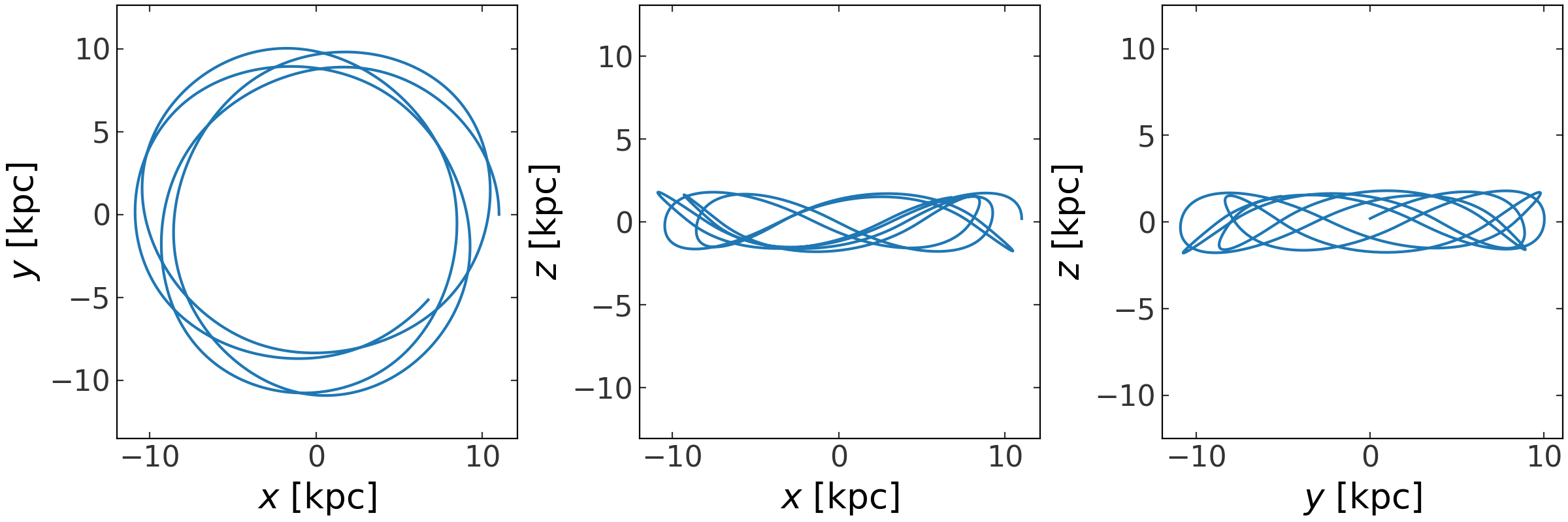
The Orbit object that is returned contains many useful methods, and can be passed to many of the analysis functions implemented in Gala. For example, we can easily visualize the orbit by plotting the time series in all Cartesian projections using the plot() method:

>>> fig = orbit.plot()

(Source code, png, pdf)

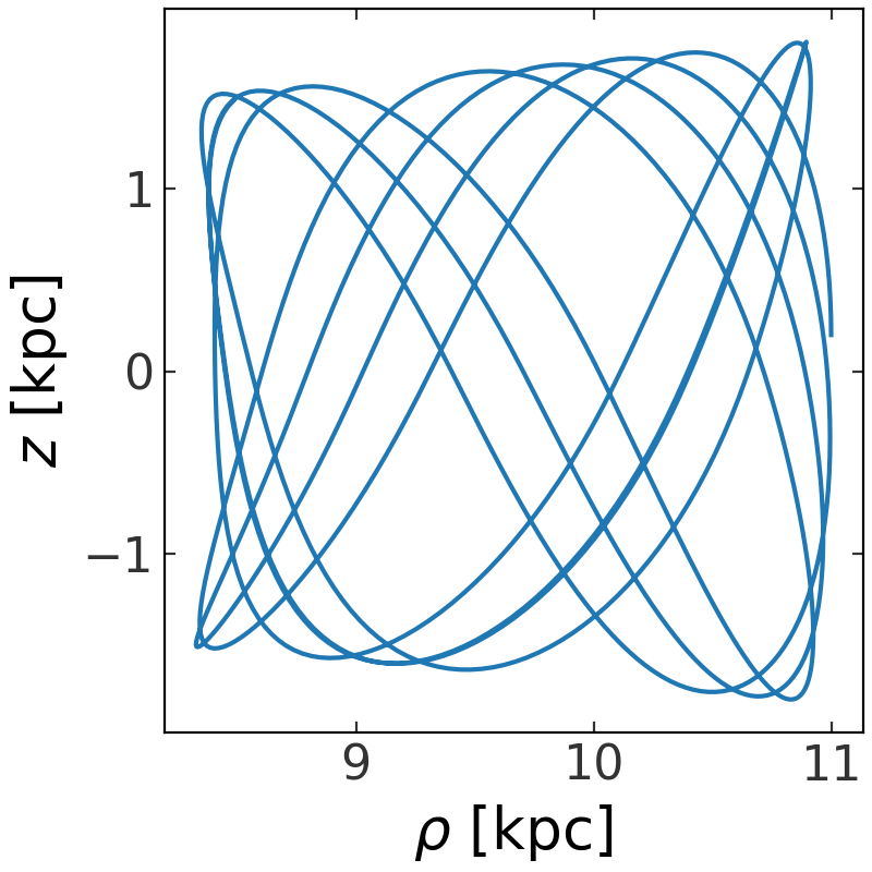
We can also visualize the orbit in transformed coordinates, for example, cylindrical radius \(\rho\) and \(z\):

>>> fig = orbit.represent_as("cylindrical").plot(["rho", "z"])

(Source code, png, pdf)

The Orbit object also enables computing dynamical quantities such as energy or angular momentum:

>>> E = orbit.energy()
>>> E[0]
<Quantity −0.060740198 kpc2 / Myr2>

Let’s check how well the integrator conserves energy and the z component of angular momentum:

>>> Lz = orbit.angular_momentum()[2]
>>> np.std(E), np.std(Lz)
(<Quantity 4.654233175716351e-06 kpc2 / Myr2>,
 <Quantity 9.675900603446092e-16 kpc2 / Myr>)

We can access the position and velocity components of the orbit separately using attributes that map to the underlying BaseRepresentation and BaseDifferential subclass instances that store the position and velocity data. The attribute names depend on the representation. For example, for a Cartesian representation, the position components are ["x", "y", "z"] and the velocity components are ["v_x", "v_y", "v_z"]. With a Orbit or PhaseSpacePosition instance, you can check the valid compnent names using the attributes .pos_components and .vel_components:

>>> orbit.pos_components.keys()
odict_keys(["x", "y", "z"])
>>> orbit.vel_components.keys()
odict_keys(["v_x", "v_y", "v_z"])

Meaning, we can access these components by doing, e.g.:

>>> orbit.v_x
<Quantity [ 0.        , -0.00567589, -0.01129934, ...,  0.18751756,
            0.18286687,  0.17812762] kpc / Myr>

For a Cylindrical representation, these are instead:

>>> cyl_orbit = orbit.represent_as("cylindrical")
>>> cyl_orbit.pos_components.keys()
odict_keys(["rho", "phi", "z"])
>>> cyl_orbit.vel_components.keys()
odict_keys(["v_rho", "pm_phi", "v_z"])
>>> cyl_orbit.v_rho
<Quantity [ 0.        , -0.00187214, -0.00369183, ...,  0.01699321,
            0.01930216,  0.02159477] kpc / Myr>

Continue to the Orbit and phase-space position objects in more detail page for more information.

Using gala.dynamics

More details are provided in the linked pages below:

• Orbit and phase-space position objects in more detail
  • Introduction
  • Phase-space Positions
  • Orbits
  • More information
• N-dimensional representation classes
  • Introduction
• Transforming to actions, angles, and frequencies
  • Introduction
  • The O2GF action solver
  • Using the Staeckel Fudge in Galpy
  • References
• Generating mock stellar streams
  • Introduction
  • Getting started
  • Self-gravity of the progenitor
  • Integration methods and options
  • Generating a stream from the present-day progenitor location
  • References
• Nonlinear Dynamics
  • Introduction
  • Computing Lyapunov exponents
• N-body (gala.dynamics.nbody)
  • Introduction
  • Getting started
  • Example: Mixed test particle and massive particle orbit integration
  • Example: N-body integration with a background potential

API

gala.dynamics Package

Classes

Orbit(pos, vel[, t, hamiltonian, potential, ...])	Represents an orbit: positions and velocities (conjugate momenta) as a function of time.
PhaseSpacePosition(pos[, vel, frame, copy])	Represents phase-space positions, i.e. positions and conjugate momenta (velocities).