%matplotlib inline

Compute a Galactic orbit for a star using Gaia data

In this tutorial, we will retrieve the sky coordinates, astrometry, and radial velocity for a star — Kepler-444 — and compute its orbit in the default Milky Way mass model implemented in Gala. We will compare the orbit of Kepler-444 to the orbit of the Sun.

Notebook Setup and Package Imports

import astropy.coordinates as coord
import astropy.units as u
import matplotlib.pyplot as plt
from pyia import GaiaData

# Gala
import gala.dynamics as gd
import gala.potential as gp

Define a Galactocentric Coordinate Frame

We will start by defining a Galactocentric coordinate system using astropy.coordinates by adopting the latest parameter set for the Solar position and velocity with respect to the Galactic Center implemented in Astropy.

with coord.galactocentric_frame_defaults.set("v4.0"):
    galcen_frame = coord.Galactocentric()
galcen_frame

<Galactocentric Frame (galcen_coord=<ICRS Coordinate: (ra, dec) in deg
    (266.4051, -28.936175)>, galcen_distance=8.122 kpc, galcen_v_sun=(12.9, 245.6, 7.78) km / s, z_sun=20.8 pc, roll=0.0 deg)>

Define the Solar Position and Velocity

In this coordinate system, the sun is along the \(x\)-axis (at a negative \(x\) value), and the Galactic rotation at this position is in the \(+y\) direction. In this coordinate system, the 3D position of the sun is therefore given by:

sun_xyz = u.Quantity(
    [-galcen_frame.galcen_distance, 0 * u.kpc, galcen_frame.z_sun]  # x  # y  # z
)

We can combine this with the solar velocity vector (set on the astropy.coordinates.Galactocentric frame) to define the sun’s phase-space position, which we will use as initial conditions shortly to compute the orbit of the Sun:

sun_w0 = gd.PhaseSpacePosition(pos=sun_xyz, vel=galcen_frame.galcen_v_sun)

To compute the sun’s orbit, we need to specify a mass model for the Galaxy. Here, we will use the same default, four-component Milky Way mass model introduced in Defining a Milky Way model:

mw_potential = gp.MilkyWayPotential()

We can now compute the Sun’s orbit using the default integrator (Leapfrog integration): We will compute the orbit for 4 Gyr, which is about 16 orbital periods:

sun_orbit = mw_potential.integrate_orbit(sun_w0, dt=0.5 * u.Myr, t1=0, t2=4 * u.Gyr)

Retrieve Gaia Data for Kepler-444

For our comparison star, we will use the exoplanet-hosting star Kepler-444. To get Gaia data for this source, we first have to retrieve its sky coordinates so that we can do a positional cross-match query on the Gaia catalog. We can retrieve the sky position of Kepler-444 using the SkyCoord.from_name() classmethod, which queries Simbad under the hood to resolve the name:

star_sky_c = coord.SkyCoord.from_name("Kepler-444")
star_sky_c

<SkyCoord (ICRS): (ra, dec) in deg
    (289.75228708, 41.63460623)>

We happen to know a priori that Kepler-444 has a large proper motion, so the sky position reported by Simbad (unknown epoch) could be off from the Gaia sky position (epoch=2016) by many arcseconds. To run and retrieve the Gaia data, we will use the pyia package: We can pass in an ADQL query, which pyia uses to query the Gaia science archive using astroquery, and returns the data as a pyia object that understands how to convert the Gaia data columns into a astropy.coordinates.SkyCoord object. To run the query, we will do a large sky position cross-match (with a radius of 15 arcseconds), and take the brightest cross-matched source within this region:

star_gaia = GaiaData.from_query(
    f"""
    SELECT TOP 1 * FROM gaiadr3.gaia_source
    WHERE 1=CONTAINS(
        POINT('ICRS', {star_sky_c.ra.degree}, {star_sky_c.dec.degree}),
        CIRCLE('ICRS', ra, dec, {(15*u.arcsec).to_value(u.degree)})
    )
    ORDER BY phot_g_mean_mag
    """
)
star_gaia

<GaiaData: 1 rows>

We will assume (and hope!) that this source is Kepler-444, but we know that it is fairly bright compared to a typical Gaia source, so we should be safe.

We can now use the returned pyia.GaiaData object to convert the Gaia astrometric and radial velocity measurements into an Astropy SkyCoord object (with all position and velocity data):

star_gaia_c = star_gaia.get_skycoord()

To compute this star’s Galactic orbit, we need to convert its observed, Heliocentric (actually solar system barycentric) data into the Galactocentric coordinate frame we defined above. To do this, we will use the astropy.coordinates transformation framework:

star_galcen = star_gaia_c.transform_to(galcen_frame)
star_galcen

<SkyCoord (Galactocentric: galcen_coord=<ICRS Coordinate: (ra, dec) in deg
    (266.4051, -28.936175)>, galcen_distance=8.122 kpc, galcen_v_sun=(12.9, 245.6, 7.78) km / s, z_sun=20.8 pc, roll=0.0 deg): (x, y, z) in pc
    [(-8111.74969996, 34.13942928, 28.92842808)]
 (v_x, v_y, v_z) in km / s
    [(71.37746301, 119.4088628, -78.91847692)]>

Now with Galactocentric position and velocity components for Kepler-444, we can create Gala initial conditions and compute its orbit on the time grid used to compute the Sun’s orbit above:

star_w0 = gd.PhaseSpacePosition(star_galcen.data)
star_orbit = mw_potential.integrate_orbit(star_w0, t=sun_orbit.t)

fig, axes = plt.subplots(1, 2, figsize=(10, 5), constrained_layout=True)

sun_orbit.plot(["x", "y"], axes=axes[0])
star_orbit.plot(["x", "y"], axes=axes[0])
axes[0].set_xlim(-10, 10)
axes[0].set_ylim(-10, 10)

sun_orbit.cylindrical.plot(
    ["rho", "z"],
    axes=axes[1],
    auto_aspect=False,
    labels=["$R$ [kpc]", "$z$ [kpc]"],
    label="Sun",
)
star_orbit.cylindrical.plot(
    ["rho", "z"],
    axes=axes[1],
    auto_aspect=False,
    labels=["$R$ [kpc]", "$z$ [kpc]"],
    label="Kepler-444",
)
axes[1].set_xlim(0, 10)
axes[1].set_ylim(-5, 5)
axes[1].set_aspect("auto")
axes[1].legend(loc="best", fontsize=15)

<matplotlib.legend.Legend at 0x7fca135843a0>

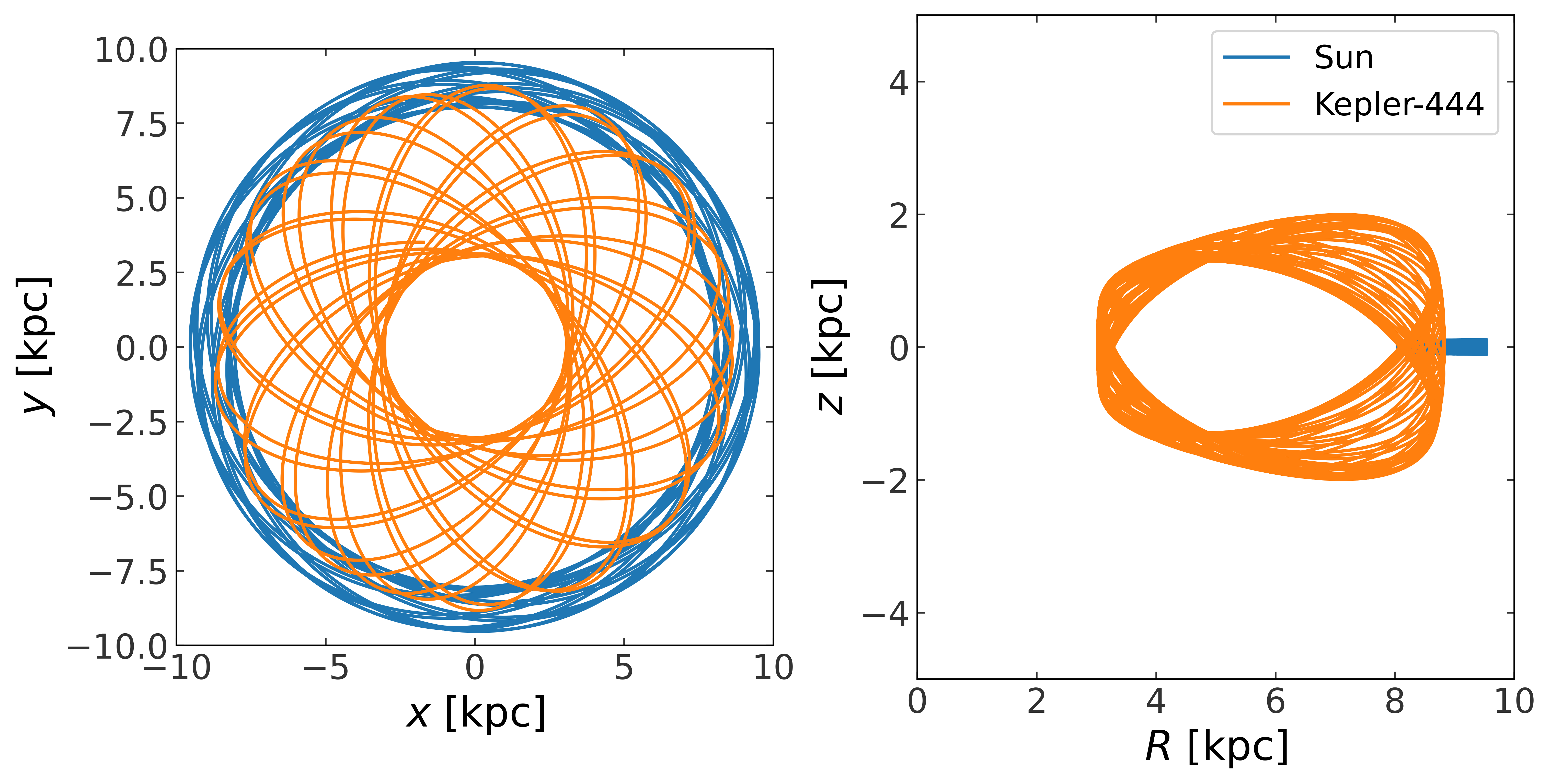
Exercise: How does Kepler-444’s orbit differ from the Sun’s?

What is the maximum \(z\) height reached by each orbit? What are their eccentricities? What are the guiding center radii of the two orbits? Can you guess which star is older based on their kinematics? Which star do you think has a higher metallicity?

Exercise: Comparing these orbits to the orbits of other Gaia stars

Retrieve Gaia data for a set of 100 random Gaia stars within 200 pc of the sun with measured radial velocities and well-measured parallaxes using the query:

SELECT TOP 100 * FROM gaiadr3.gaia_source
    WHERE radial_velocity IS NOT NULL AND
        parallax_over_error > 10 AND
        ruwe < 1.2 AND
        parallax > 5
    ORDER BY random_index

random_stars_g = GaiaData.from_query(
    """
    SELECT TOP 100 * FROM gaiadr3.gaia_source
    WHERE radial_velocity IS NOT NULL AND
        parallax_over_error > 10 AND
        ruwe < 1.2 AND
        parallax > 5
    ORDER BY random_index
    """
)

Compute orbits for these stars for the same time grid used above to compute the sun’s orbit:

random_stars_c = random_stars_g.get_skycoord()

random_stars_galcen = random_stars_c.transform_to(galcen_frame)
random_stars_w0 = gd.PhaseSpacePosition(random_stars_galcen.data)

random_stars_orbits = mw_potential.integrate_orbit(random_stars_w0, t=sun_orbit.t)

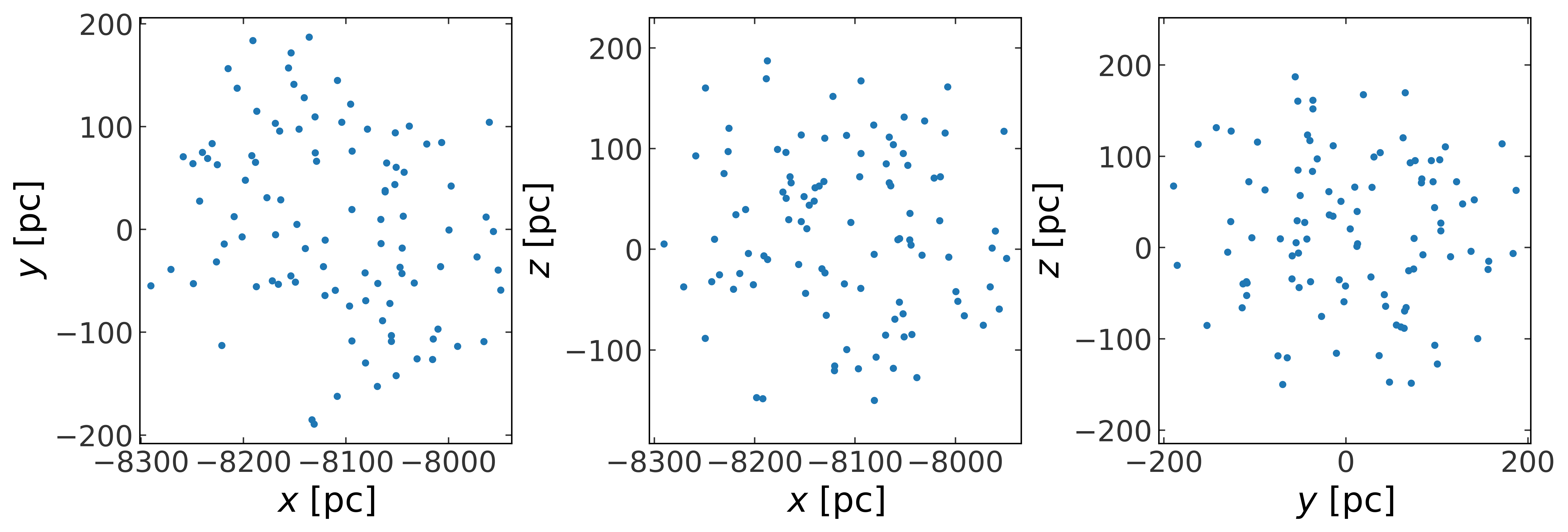
Plot the initial (present-day) positions of all of these stars in Galactocentric Cartesian coordinates:

_ = random_stars_w0.plot()

Plot the orbits of these stars in the x-y and R-z planes:

fig, axes = plt.subplots(1, 2, figsize=(10, 5), constrained_layout=True)

random_stars_orbits.plot(["x", "y"], axes=axes[0])
axes[0].set_xlim(-15, 15)
axes[0].set_ylim(-15, 15)

random_stars_orbits.cylindrical.plot(
    ["rho", "z"],
    axes=axes[1],
    auto_aspect=False,
    labels=["$R$ [kpc]", "$z$ [kpc]"],
)

axes[1].set_xlim(0, 15)
axes[1].set_ylim(-5, 5)
axes[1].set_aspect("auto")

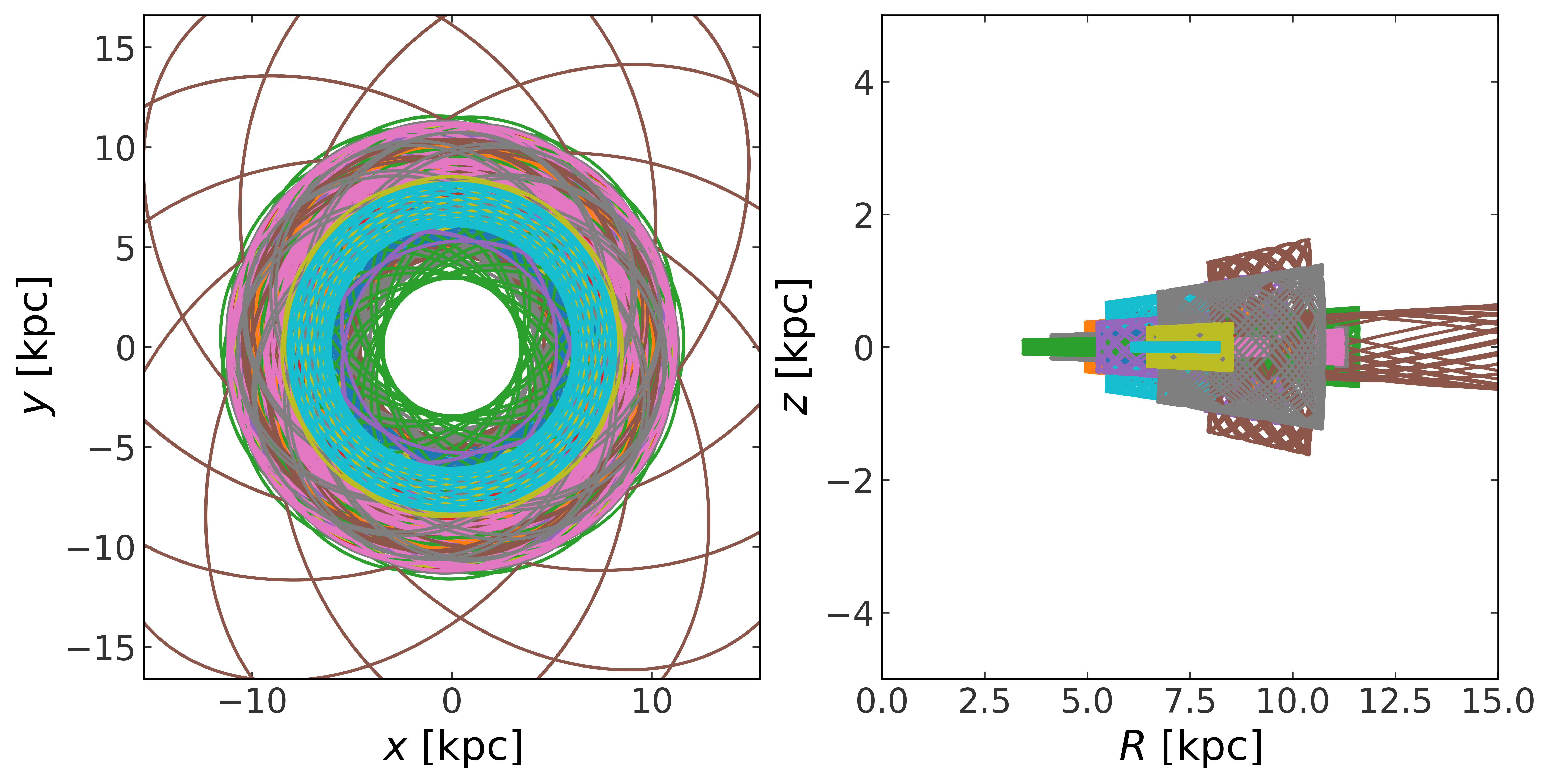
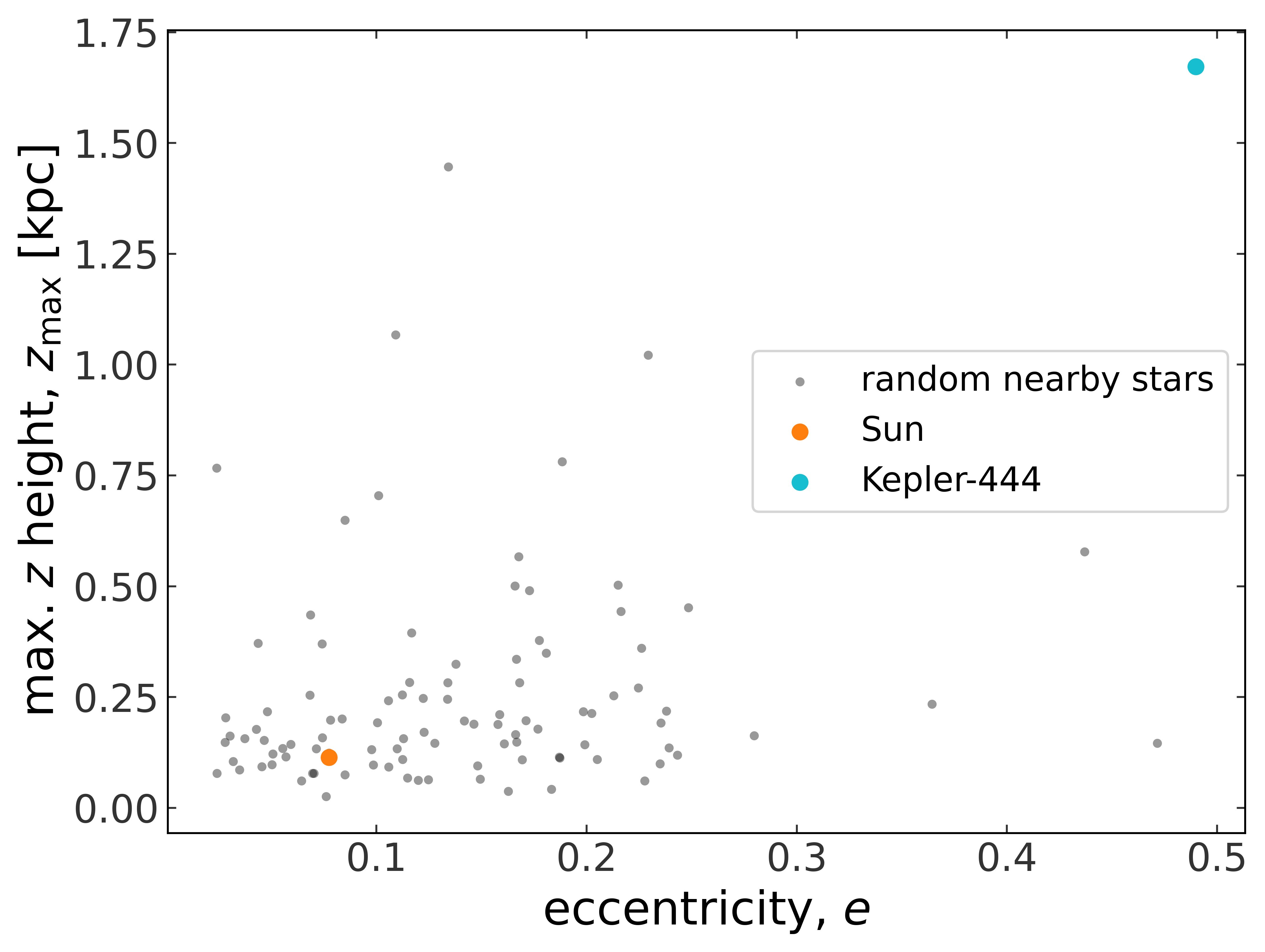
Compute maximum \(z\) heights (\(z_\textrm{max}\)) and eccentricities for all of these orbits. Compare the Sun, Kepler-444, and this random sampling of nearby stars. Where do the Sun and Kepler-444 sit relative to the random sample of nearby stars in terms of \(z_\textrm{max}\) and eccentricity? (Hint: plot \(z_\textrm{max}\) vs. eccentricity and highlight the Sun and Kepler-444!) Are either of them outliers in any way?

rand_zmax = random_stars_orbits.zmax()

rand_ecc = random_stars_orbits.eccentricity()

fig, ax = plt.subplots(figsize=(8, 6))
ax.scatter(
    rand_ecc, rand_zmax, color="k", alpha=0.4, s=14, lw=0, label="random nearby stars"
)
ax.scatter(sun_orbit.eccentricity(), sun_orbit.zmax(), color="tab:orange", label="Sun")
ax.scatter(
    star_orbit.eccentricity(), star_orbit.zmax(), color="tab:cyan", label="Kepler-444"
)
ax.legend(loc="best", fontsize=14)
ax.set_xlabel("eccentricity, $e$")
ax.set_ylabel(r"max. $z$ height, $z_{\rm max}$ [kpc]")

Text(0, 0.5, 'max. $z$ height, $z_{\\rm max}$ [kpc]')