Nonlinear Dynamics#
Introduction#
This module contains utilities for nonlinear dynamics. Currently, the only implemented features enable you to compute estimates of the maximum Lyapunov exponent for an orbit. In future releases, there will be features for creating surface of sections and computing the full Lyapunov spectrum.
Some imports needed for the code below:
>>> import astropy.units as u
>>> import numpy as np
>>> import gala.potential as gp
>>> import gala.dynamics as gd
>>> from gala.units import galactic
Computing Lyapunov exponents#
Chaotic orbit#
There are two ways to compute Lyapunov exponents implemented in gala.dynamics.
In most cases, you’ll want to use the
fast_lyapunov_max function because the integration is
implemented in C and is quite fast. This function only works if the potential
you are working with is implemented in C (e.g., it is a
CPotentialBase subclass). With a potential object
and a set of initial conditions:
>>> pot = gp.LogarithmicPotential(v_c=150*u.km/u.s, r_h=0.1*u.kpc,
...                               q1=1., q2=0.8, q3=0.6, units=galactic)
>>> w0 = gd.PhaseSpacePosition(pos=[5.5,0.,5.5]*u.kpc,
...                            vel=[0.,100.,0]*u.km/u.s)
>>> lyap,orbit = gd.fast_lyapunov_max(w0, pot, dt=2., n_steps=100000)
This returns two objects: an Quantity object that
contains the maximum Lyapunov exponent estimate for each offset orbit,
(we can control the number of offset orbits with the noffset_orbits
argument) and an Orbit object that contains
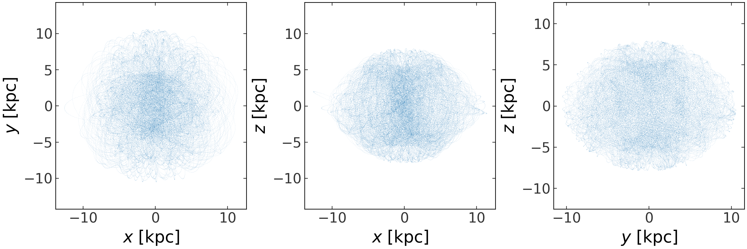
the parent orbit and each offset orbit. Let’s plot the parent orbit:
>>> fig = orbit[:,0].plot(marker=',', alpha=0.25, linestyle='none')
(Source code, png, pdf)

Visually, this looks like a chaotic orbit. This means the Lyapunov exponent
should saturate to some value. We’ll now plot the estimate of the Lyapunov
exponent as a function of time – because the algorithm re-normalizes every
several time-steps (controllable with the n_steps_per_pullback argument),
we have to down-sample the time array to align it with the Lyapunov exponent
array. This plots one line per offset orbit:
>>> plt.figure()
>>> plt.loglog(orbit.t[11::10], lyap, marker='')
>>> plt.xlabel("Time [{}]".format(orbit.t.unit))
>>> plt.ylabel(r"$\lambda_{{\rm max}}$ [{}]".format(lyap.unit))
>>> plt.tight_layout()
(Source code, png, pdf)
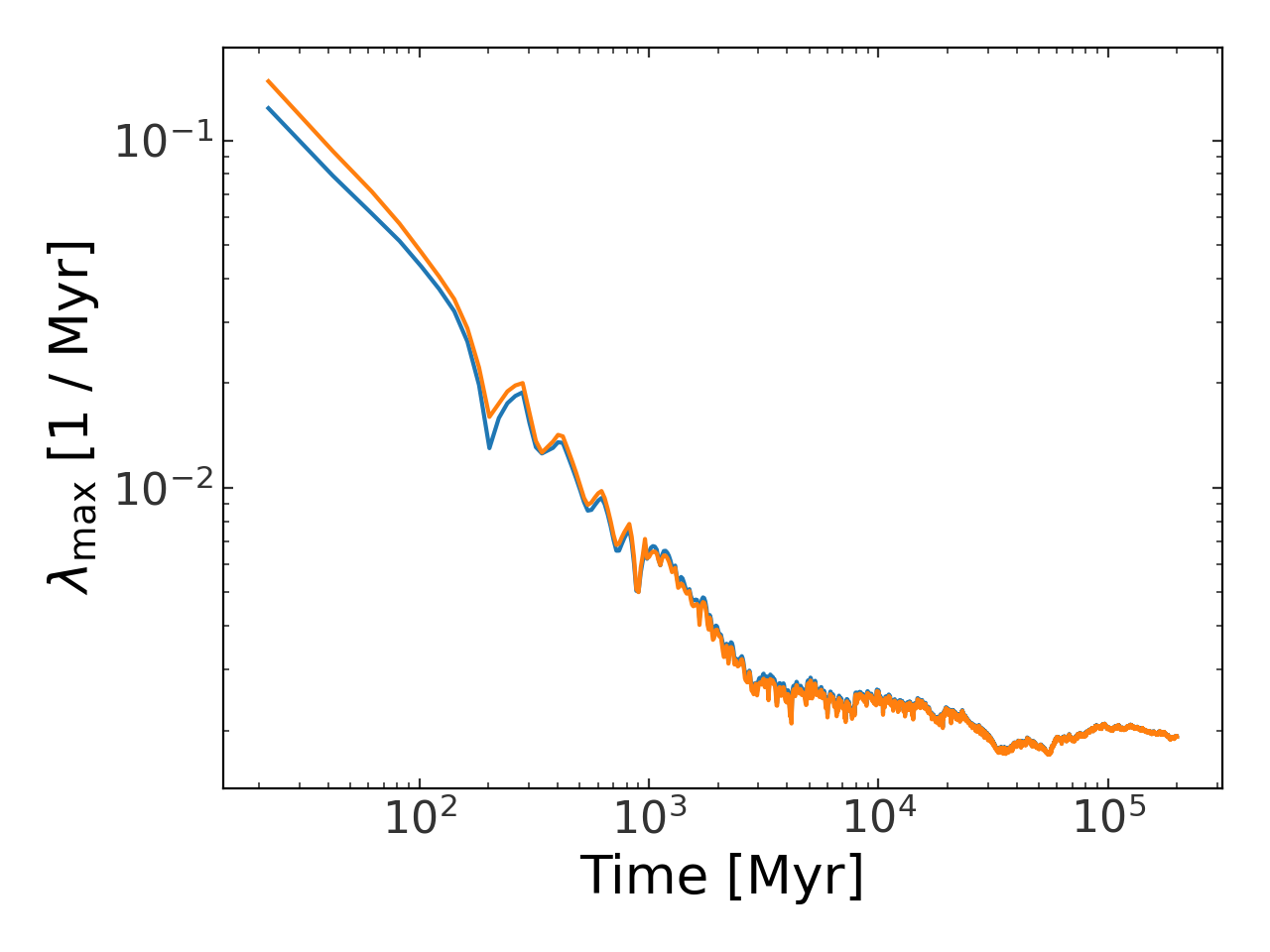
The estimate is clearly starting to diverge from a simple power law decay.
Regular orbit#
To compare, we will compute the estimate for a regular orbit as well:
>>> w0 = gd.PhaseSpacePosition(pos=[5.5,0.,0.]*u.kpc,
...                            vel=[0.,140.,25]*u.km/u.s)
>>> lyap,orbit = gd.fast_lyapunov_max(w0, pot, dt=2., n_steps=100000)
>>> fig = orbit[:,0].plot(marker=',', alpha=0.1, linestyle='none')
(Source code, png, pdf)
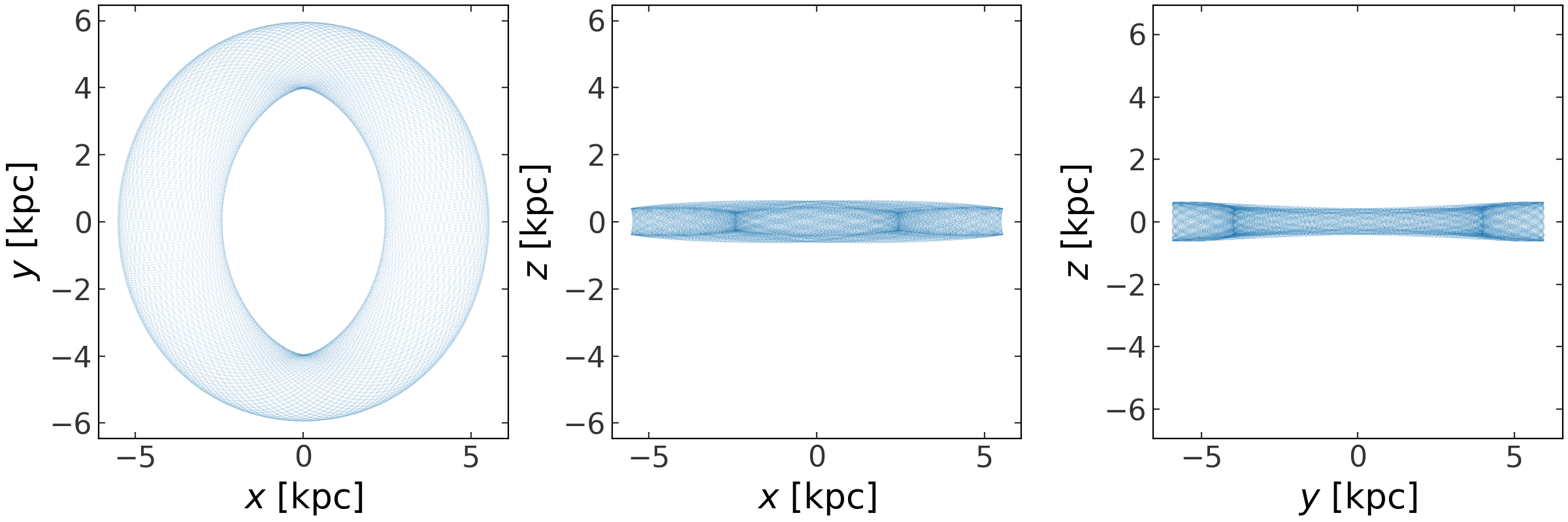
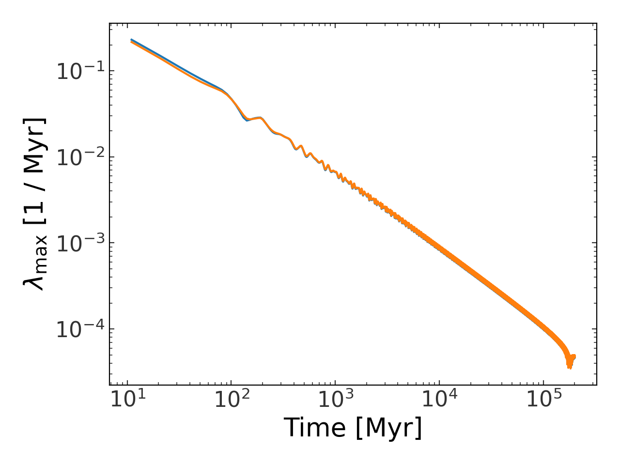
Because this is a regular orbit, the estimate continues decreasing, following a characteristic power-law (a straight line in a log-log plot):
>>> pl.figure()
>>> pl.loglog(orbit.t[11::10], lyap, marker='')
>>> pl.xlabel("Time [{}]".format(orbit.t.unit))
>>> pl.ylabel(r"$\lambda_{{\rm max}}$ [{}]".format(lyap.unit))
>>> pl.tight_layout()
(Source code, png, pdf)
API#
Functions#
|
Compute the maximum Lyapunov exponent using a C-implemented estimator that uses the DOPRI853 integrator. |
|
Compute the maximum Lyapunov exponent of an orbit by integrating many nearby orbits ( |
|
Generate and return a surface of section from the given orbit. |