Generating a mock stellar stream and converting to Heliocentric coordinates
We first need to import some relevant packages:
>>> import astropy.coordinates as coord
>>> import astropy.units as u
>>> import numpy as np
>>> import gala.coordinates as gc
>>> import gala.dynamics as gd
>>> import gala.potential as gp
>>> from gala.units import galactic
In the examples below, we will use the galactic
UnitSystem: as I define it, this is: \({\rm kpc}\),
\({\rm Myr}\), \({\rm M}_\odot\).
We first create a potential object to work with. For this example, we’ll use a two-component potential: a Miyamoto-Nagai disk with a spherical NFW potential to represent a dark matter halo.
>>> pot = gp.CCompositePotential()
>>> pot['disk'] = gp.MiyamotoNagaiPotential(m=6E10*u.Msun,
...                                         a=3.5*u.kpc, b=280*u.pc,
...                                         units=galactic)
>>> pot['halo'] = gp.NFWPotential(m=1E12, r_s=20*u.kpc, units=galactic)
We’ll use the Palomar 5 globular cluster and stream as a motivation for this example. For the position and velocity of the cluster, we’ll use \((\alpha, \delta) = (229, −0.124)~{\rm deg}\) [odenkirchen02], \(d = 22.9~{\rm kpc}\) [bovy16], \(v_r = -58.7~{\rm km}~{\rm s}^{-1}\) [bovy16], and \((\mu_{\alpha,*}, \mu_\delta) = (-2.296,-2.257)~{\rm mas}~{\rm yr}^{-1}\) [fritz15]:
>>> c = coord.ICRS(ra=229 * u.deg, dec=-0.124 * u.deg,
...                distance=22.9 * u.kpc,
...                pm_ra_cosdec=-2.296 * u.mas/u.yr,
...                pm_dec=-2.257 * u.mas/u.yr,
...                radial_velocity=-58.7 * u.km/u.s)
We’ll first convert this position and velocity to Galactocentric coordinates:
>>> c_gc = c.transform_to(coord.Galactocentric).cartesian
>>> c_gc
<CartesianRepresentation (x, y, z) in kpc
    (7.69726478, 0.22748727, 16.41135761)
 (has differentials w.r.t.: 's')>
>>> pal5 = gd.PhaseSpacePosition(pos=c_gc.xyz, vel=c_gc.differentials['s'].d_xyz)
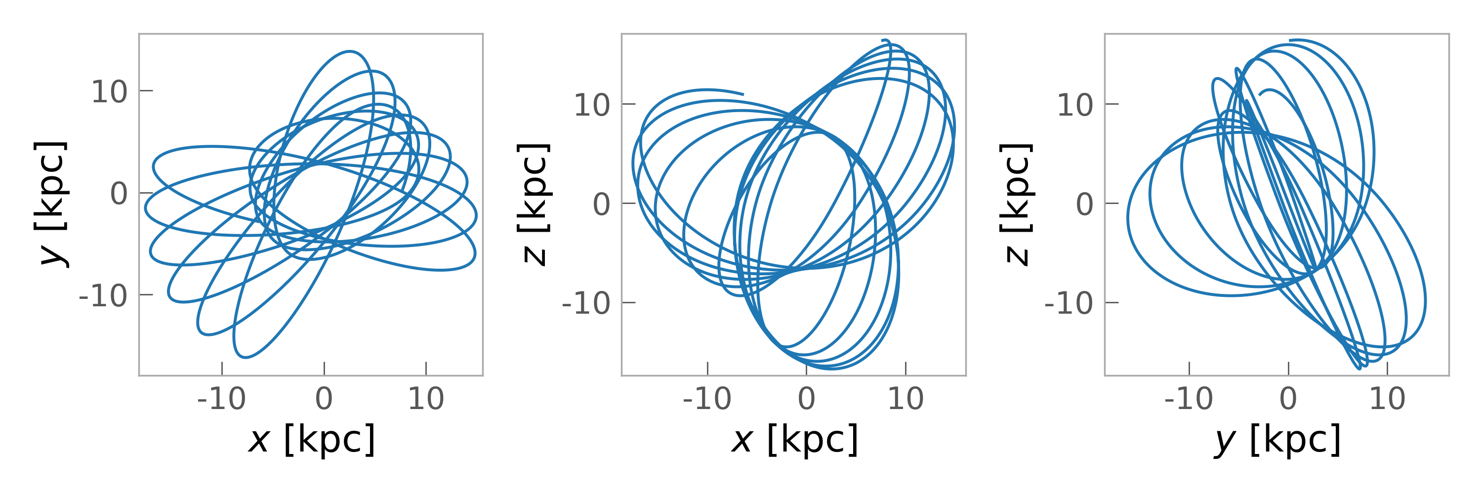
We can now integrate an orbit in the previously defined gravitational potential using Pal 5’s position and velocity as initial conditions. We’ll integrate the orbit backwards (using a negative time-step) from its present-day position for 4 Gyr:
>>> pal5_orbit = gp.Hamiltonian(pot).integrate_orbit(pal5, dt=-0.5*u.Myr, n_steps=8000)
>>> fig = pal5_orbit.plot()
(Source code, png)
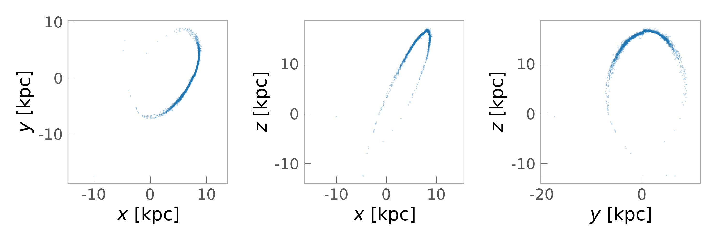
We can now generate a mock stellar stream using the orbit of the progenitor system (the Pal 5 cluster). We’ll generate a stream using the prescription presented in [fardal15]:
>>> from gala.dynamics.mockstream import fardal_stream
>>> stream = fardal_stream(pot, pal5_orbit[::-1], prog_mass=1E5*u.Msun,
...                        release_every=4)
>>> fig = stream.plot(marker='.', s=1, alpha=0.25)
(Source code, png)

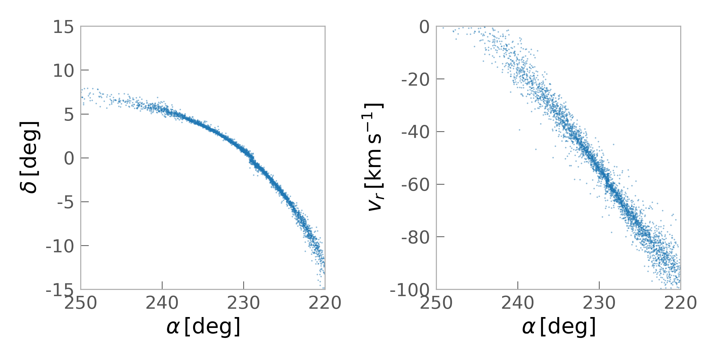
We now have the model stream particle positions and velocities in a Galactocentric coordinate frame. To convert these to observable, Heliocentric coordinates, we have to specify a desired coordinate frame. We’ll convert to the ICRS coordinate system and plot some of the Heliocentric kinematic quantities:
>>> stream_c = stream.to_coord_frame(coord.ICRS)
(Source code, png)

References
| [odenkirchen02] | Odenkirchen et al. (2002) |
| [fritz15] | Fritz & Kallivayali (2015) |
| [bovy16] | (1, 2) Bovy et al. (2016) |