Generating mock stellar streams

Introduction

This module contains functions for generating mock stellar streams using a variety of methods that approximate the formation of streams in N-body simulations.

Some imports needed for the code below:

>>> import astropy.units as u
>>> import numpy as np
>>> import gala.potential as gp
>>> import gala.dynamics as gd
>>> from gala.dynamics.mockstream import mock_stream
>>> from gala.units import galactic

Warning

The API for this subpackage is experimental and may change in a future release. This code has not been tested extensively – feedback is welcome!

Model parametrization

The core implementation follows the parametrization used by [fardal15] (except where noted below), which outlines a general way to specify the position and velocity distributions of stars stripped from the progenitor system at the time of stripping. In cylindrical coordinates \((R,\phi,z)\) in the orbital plane of the progenitor system (at position \((R_p,\phi_p,z_p)\)) the position of the \(i\) th star at the time it is stripped from the satellite is given by:

\[\begin{split}R_i &= R_p \pm k_R\,r_{\rm tide}\\ \phi_i &= \phi_p + k_\phi\,\frac{r_{\rm tide}}{R_p}\\ z_i &= k_z\,r_{\rm tide}\end{split}\]

where \(r_{\rm tide}\) is the tidal radius and the parameters \((k_R,k_\phi,k_z)\) allow completely general specification of the distribution of stripped stars (e.g., they may be constants, drawn from probability distributions, functions of time). Similarly, in velocity:

\[\begin{split}v_{R,i} &= v_{R,p} + k_{vR}\,v_{R,p}\\ v_{\phi,i} &= v_{\phi,p} + k_{v\phi}\,\Omega_p\,k_R\,r_{\rm tide}\\ v_{z,i} &= v_{z,p} + k_{vz}\,\Omega_p\,r_{\rm tide}\end{split}\]

where \(\Omega_p\) is the orbital frequency of the progenitor.

Because this framework is very general, we can use it to reproduce many of the methods that have been used in the literature. Two examples are included below: the Streakline method from [kuepper12] and the method from [fardal15].

Note

The method outlined above allows for arbitrary mass-loss histories or distributions of stripping times, however, currently only uniform mass-loss is supported.

Streakline streams

In the Streakline method, star particles are released with the same angular velocity as the satellite at the tidal radius with no dispersion. This is equivalent to fixing the \(k\) parameters to:

\[\begin{split}k_R &= 1.\\ k_{v\phi} &= 1.\\ k_\phi &= k_z = k_{vR} = k_{vz} = 0\end{split}\]

We can set these parameters when generating a stream model with mock_stream, but first we need to specify a potential and integrate the orbit of the progenitor system. We’ll use a spherical NFW potential, a progenitor mass \(m=10^4~{\rm M}_\odot\) and initial conditions that place the progenitor on a mildly eccentric orbit:

>>> pot = gp.NFWPotential.from_circular_velocity(v_c=250*u.km/u.s,
...                                              r_s=10*u.kpc,
...                                              units=galactic)
>>> prog_mass = 1E4*u.Msun
>>> prog_w0 = gd.PhaseSpacePosition(pos=[15, 0, 0.]*u.kpc,
...                                 vel=[75, 150, 30.]*u.km/u.s)
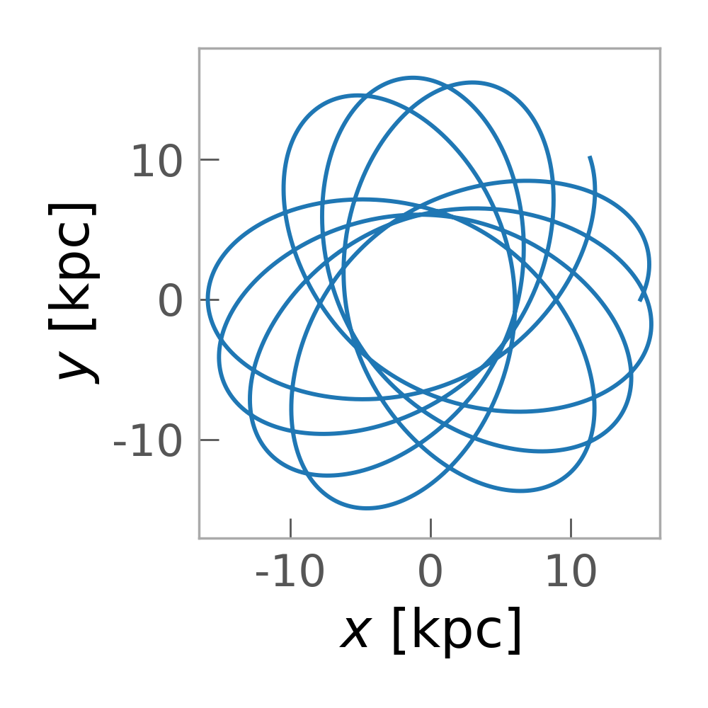
>>> prog_orbit = gp.Hamiltonian(pot).integrate_orbit(prog_w0, dt=0.5, n_steps=4000)
>>> fig = prog_orbit.plot(['x', 'y'])

(Source code, png)

We now have to define the k parameters. This is done by defining an iterable with 6 elements corresponding to \((k_R, k_\phi, k_z, k_{vR}, k_{v\phi}, k_{vz})\). We also have to set the dispersions in these parameters to 0.

>>> k_mean = [1., 0, 0, 0, 1., 0]
>>> k_disp = np.zeros(6)

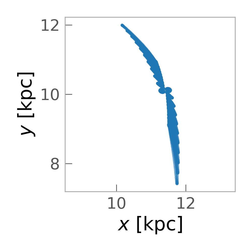
Now we generate the mock stream. We will release a star particle every time-step from both Lagrange points by setting release_every=1:

>>> stream = mock_stream(pot, prog_orbit, prog_mass,
...                      k_mean=k_mean, k_disp=k_disp, release_every=1)
>>> fig = stream.plot(['x', 'y'], marker='.', alpha=0.25)

(Source code, png)

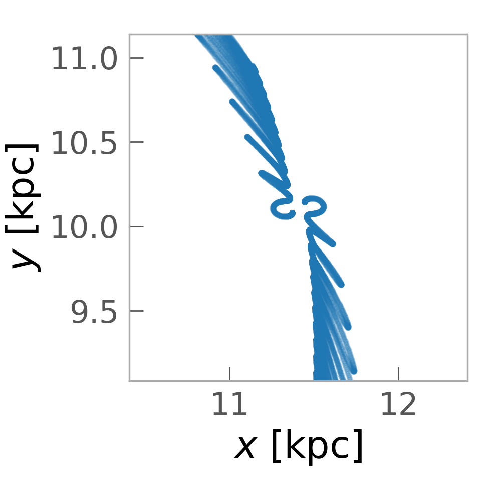
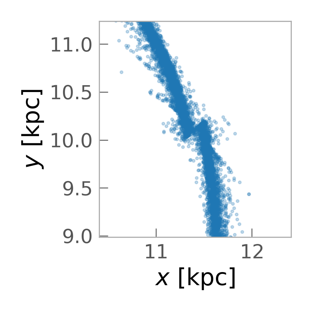
Or, zooming in around the progenitor:

(Source code, png)

Fardal streams

[fardal15] found values for the k parameters and their dispersions by matching to N-body simulations. For this method, these are set to:

>>> k_mean = [2., 0, 0, 0, 0.3, 0]
>>> k_disp = [0.5, 0, 0.5, 0, 0.5, 0.5]

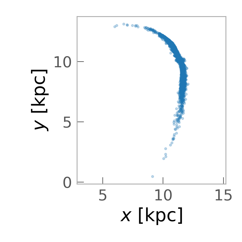
With the same potential and progenitor orbit as above, we now generate a mock stream using this method:

>>> stream2 = mock_stream(pot, prog_orbit, prog_mass,
...                       k_mean=k_mean, k_disp=k_disp,
...                       release_every=1)
>>> fig = stream2.plot(['x', 'y'], marker='.', alpha=0.25)

(Source code, png)

Or, again, zooming in around the progenitor:

(Source code, png)

References

[fardal15]

(1, 2, 3) Fardal, Huang, Weinberg (2015)

[kuepper12]

Küpper, Lane, Heggie (2012)

API

Functions

dissolved_fardal_stream(hamiltonian, …[, …])	Generate a mock stellar stream in the specified potential with a progenitor system that ends up at the specified position.
fardal_stream(hamiltonian, prog_orbit, prog_mass)	Generate a mock stellar stream in the specified potential with a progenitor system that ends up at the specified position.
mock_stream(hamiltonian, prog_orbit, …[, …])	Generate a mock stellar stream in the specified potential with a progenitor system that ends up at the specified position.
streakline_stream(hamiltonian, prog_orbit, …)	Generate a mock stellar stream in the specified potential with a progenitor system that ends up at the specified position.