Transforming to actions, angles, and frequencies
Introduction
Regular orbits permit a (local) transformation to a set of canonical coordinates such that the momenta are independent, isolating integrals of motion (the actions, \(\boldsymbol{J}\)) and the conjugate coordinate variables (the angles, \(\boldsymbol{\theta}\)) linearly increase time. Action-angle coordinates are useful for a number of applications because Hamilton’s equations – the equations of motion – are simple:
Analytic transformations from phase-space to action-angle coordinates are only known for a few simple cases where the gravitational potential is separable or has many symmetries. However, astronomical systems can often be triaxial or have complex radial profiles that are not captured by these simple systems. Here we have implemented the method described in [sanders14] for computing actions and angles for an arbitrary numerically integrated orbit. We demonstrate this method below with two orbits:
(see also [binneytremaine] and [mcgill90]) For the examples below, we will use
the galactic unit system and assume the following imports have
been executed:
>>> import astropy.coordinates as coord
>>> import astropy.units as u
>>> import matplotlib.pyplot as plt
>>> import numpy as np
>>> import gala.potential as gp
>>> import gala.dynamics as gd
>>> from gala.units import galactic
For many more options for action calculation, see tact.
A tube orbit in an axisymmetric potential
For an example of an axisymmetric potential, we use a flattened logarithmic potential:
with parameters
For the orbit, we use initial conditions
We first create a potential and set up our initial conditions:
>>> pot = gp.LogarithmicPotential(v_c=150*u.km/u.s, q1=1., q2=1., q3=0.9, r_h=0,
...                               units=galactic)
>>> w0 = gd.PhaseSpacePosition(pos=[8, 0, 0.]*u.kpc,
...                            vel=[75, 150, 50.]*u.km/u.s)
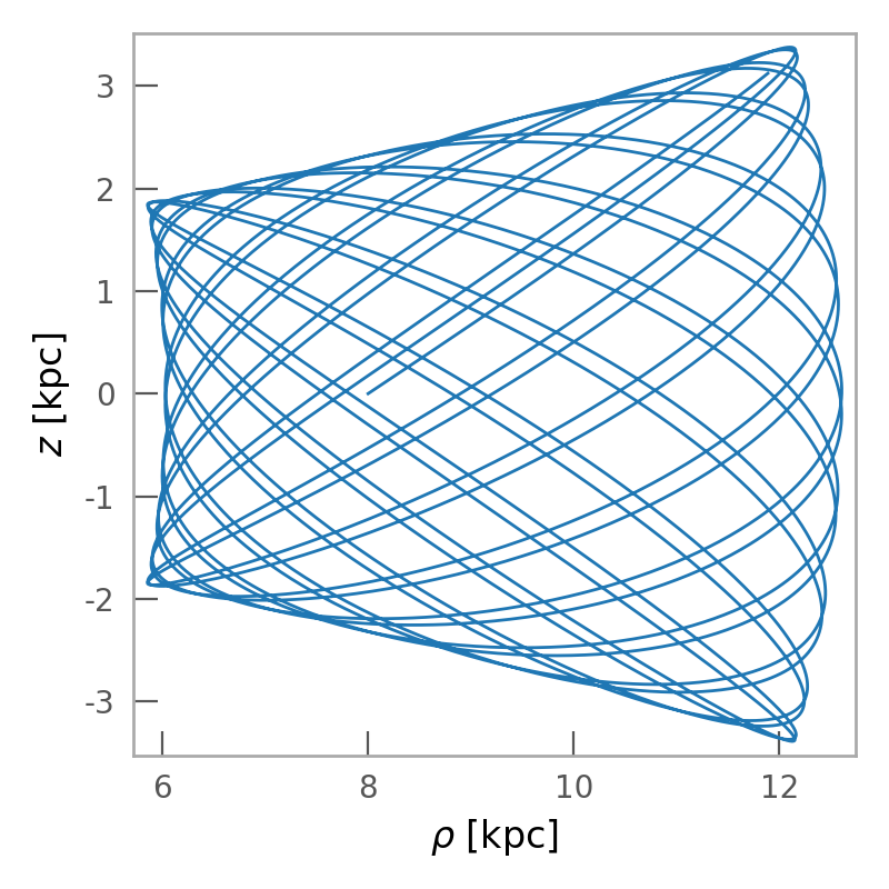
We will now integrate the orbit and plot it in the meridional plane:
>>> w = gp.Hamiltonian(pot).integrate_orbit(w0, dt=0.5, n_steps=10000)
>>> cyl = w.represent_as('cylindrical')
>>> fig = cyl.plot(['rho', 'z'], linestyle='-')
(Source code, png)
To solve for the actions in the true potential, we first compute the actions in
a “toy” potential – a potential in which we can compute the actions and angles
analytically. The two simplest potentials for which this is possible are the
IsochronePotential and
HarmonicOscillatorPotential. We will use the Isochrone
potential as our toy potential for tube orbits and the harmonic oscillator for
box orbits.
We start by finding the parameters of the toy potential (Isochrone in this case) by minimizing the dispersion in energy for the orbit:
>>> toy_potential = gd.fit_isochrone(w)
>>> toy_potential
<IsochronePotential: m=1.24e+11, b=4.02 (kpc,Myr,solMass,rad)>
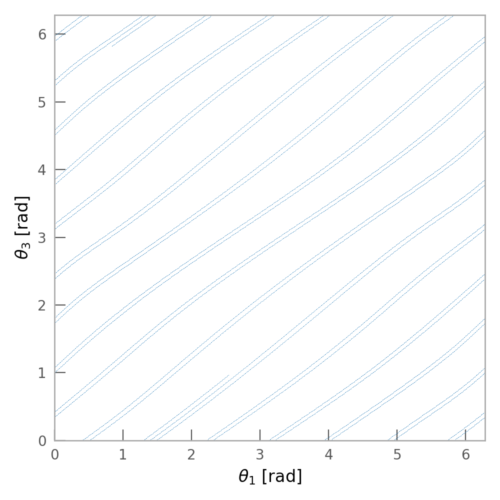
The actions and angles in this potential are not the true actions, but will only serve as an approximation. This can be seen in the angles: the orbit in the true angles would be perfectly straight lines with slope equal to the frequencies. Instead, the orbit is wobbly in the toy potential angles:
>>> toy_actions,toy_angles,toy_freqs = toy_potential.action_angle(w)
>>> fig,ax = plt.subplots(1,1,figsize=(5,5))
>>> ax.plot(toy_angles[0], toy_angles[2], linestyle='none', marker=',')
>>> ax.set_xlim(0,2*np.pi)
>>> ax.set_ylim(0,2*np.pi)
>>> ax.set_xlabel(r"$\theta_1$ [rad]")
>>> ax.set_ylabel(r"$\theta_3$ [rad]")
(Source code, png)

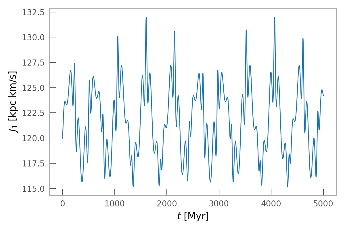
This can also be seen in the value of the action variables, which are not time-independent in the toy potential:
>>> fig,ax = plt.subplots(1,1)
>>> ax.plot(w.t, toy_actions[0], marker='')
>>> ax.set_xlabel(r"$t$ [Myr]")
>>> ax.set_ylabel(r"$J_1$ [rad]")
(Source code, png)

We can now find approximations to the actions in the true potential. We have to
choose the maximum integer vector norm, N_max, which here we arbitrarilty set
to 8. This will change depending on the convergence of the action correction
(the properties of the orbit and potential) and the accuracy desired:
>>> result = gd.find_actions(w, N_max=8, toy_potential=toy_potential)
>>> result.keys()
dict_keys(['Sn', 'nvecs', 'freqs', 'dSn_dJ', 'angles', 'actions'])
The value of the actions, frequencies, and the angles at t=0 are returned in the result dictionary:
>>> result['actions']
<Quantity [ 0.12472277, 1.22725461, 0.05847431] kpc2 solMass / Myr>
To visualize how the actions are computed, we again plot the actions in the toy potential and then plot the “corrected” actions – the approximation to the actions computed using this machinery:
>>> nvecs = gd.generate_n_vectors(8, dx=1, dy=2, dz=2)
>>> act_correction = nvecs.T[...,None] * result['Sn'][None,:,None] * np.cos(nvecs.dot(toy_angles))[None]
>>> action_approx = toy_actions - 2*np.sum(act_correction, axis=1)*u.kpc**2/u.Myr
>>>
>>> fig,ax = plt.subplots(1,1)
>>> ax.plot(w.t, toy_actions[0].to(u.km/u.s*u.kpc), marker='', label='$J_1$')
>>> ax.plot(w.t, action_approx[0].to(u.km/u.s*u.kpc), marker='', label="$J_1'$")
>>> ax.set_xlabel(r"$t$ [Myr]")
>>> ax.set_ylabel(r"[kpc ${\rm M}_\odot$ km/s]")
>>> ax.legend()
(Source code, png)
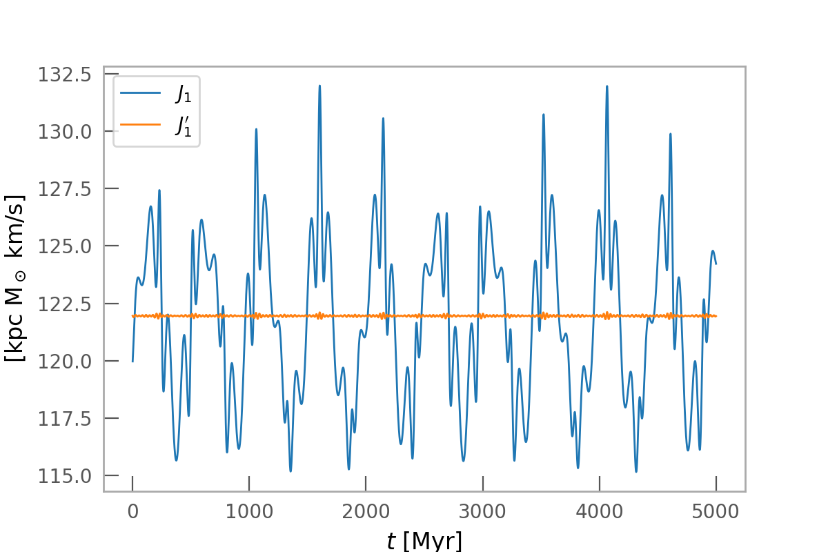
Above the blue line represents the approximation of the actions in the true potential.
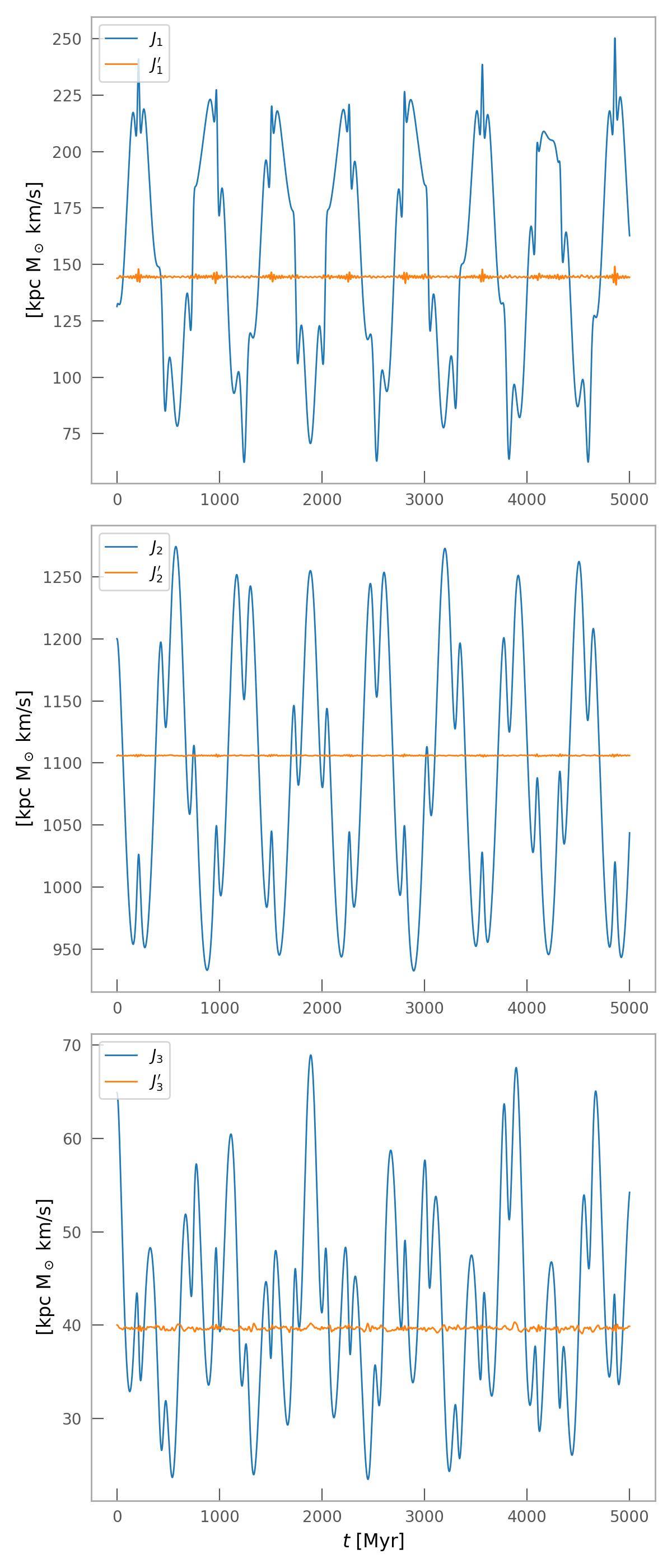
A tube orbit in a triaxial potential
The same procedure works for regular orbits in more complex potentials. We demonstrate this below by repeating the above in a triaxial potential. We again use a logarithmic potential, but with flattening along two dimensions:
with parameter values:
and the same initial conditions as above:
import astropy.coordinates as coord
import astropy.units as u
import matplotlib.pyplot as plt
import numpy as np
import gala.potential as gp
import gala.dynamics as gd
from gala.units import galactic

# define potential
pot = gp.LogarithmicPotential(v_c=150*u.km/u.s, q1=1., q2=0.9, q3=0.8, r_h=0,
                              units=galactic)

# define initial conditions
w0 = gd.PhaseSpacePosition(pos=[8, 0, 0.]*u.kpc,
                           vel=[75, 150, 50.]*u.km/u.s)

# integrate orbit
w = gp.Hamiltonian(pot).integrate_orbit(w0, dt=0.5, n_steps=10000)

# solve for toy potential parameters
toy_potential = gd.fit_isochrone(w)

# compute the actions,angles in the toy potential
toy_actions,toy_angles,toy_freqs = toy_potential.action_angle(w)

# find approximations to the actions in the true potential
import warnings
with warnings.catch_warnings(record=True):
    warnings.simplefilter("ignore")
    result = gd.find_actions(w, N_max=8, toy_potential=toy_potential)

# for visualization, compute the action correction used to transform the
#   toy potential actions to the approximate true potential actions
nvecs = gd.generate_n_vectors(8, dx=1, dy=2, dz=2)
act_correction = nvecs.T[...,None] * result['Sn'][None,:,None] * np.cos(nvecs.dot(toy_angles))[None]
action_approx = toy_actions - 2*np.sum(act_correction, axis=1)*u.kpc**2/u.Myr

fig,axes = plt.subplots(3,1,figsize=(6,14))

for i,ax in enumerate(axes):
    ax.plot(w.t, toy_actions[i].to(u.km/u.s*u.kpc), marker='', label='$J_{}$'.format(i+1))
    ax.plot(w.t, action_approx[i].to(u.km/u.s*u.kpc), marker='', label="$J_{}'$".format(i+1))
    ax.set_ylabel(r"[kpc ${\rm M}_\odot$ km/s]")
    ax.legend(loc='upper left')

ax.set_xlabel(r"$t$ [Myr]")
fig.tight_layout()
(Source code, png)

References
- sanders14
Sanders & Binney (2014) Actions, angles and frequencies for numerically integrated orbits
- binneytremaine
Binney & Tremaine (2008) Galactic Dynamics
- mcgill90
McGill & Binney (1990) Torus construction in general gravitational potentials