Generating mock stellar streams

Introduction

This module contains functions for generating mock stellar streams using a variety of methods that approximate the formation of streams in N-body simulations. Mock streams are generated by specifying time-stepping and release time information (i.e., when should stream particles be generated), and by specifying the stream distribution function (DF) to use to generate initial conditions for the stream particles. The former is customizable, and a number of popular stream DFs are implemented.

Some imports needed for the code below:

>>> import astropy.units as u
>>> import numpy as np
>>> import gala.potential as gp
>>> import gala.dynamics as gd
>>> from gala.dynamics import mockstream as ms
>>> from gala.units import galactic

We will also set the default Astropy Galactocentric frame parameters to the values adopted in Astropy v4.0:

>>> import astropy.coordinates as coord
>>> _ = coord.galactocentric_frame_defaults.set('v4.0')

Getting started

All mock stream generation done using the built-in gravitational potential models implemented in gala.potential, so we must first specify a gravitational potential to integrate orbits in. For the examples below, we will use a spherical NFW potential with a circular velocity at the scale radius of 220 km/s, and a scale radius of 15 kpc:

>>> pot = gp.NFWPotential.from_circular_velocity(v_c=220*u.km/u.s,
...                                              r_s=15*u.kpc,
...                                              units=galactic)

The mock stream generation supports any of the reference frames implemented in gala (e.g., non-static / rotating reference frames), so we must create a Hamiltonian object to use when generating streams. By default, this will use a static reference frame:

>>> H = gp.Hamiltonian(pot)

Next, we will create initial conditions for the progenitor system. In this case, we will generate the mock stream starting from this position going forward in time. However, this is customizable: if you instead have the final position of the progenitor system, there is a convenient way of doing this described below (see Generating a stream from the present-day progenitor location). Let’s specify a position and velocity that we think will produce a mildly eccentric orbit in the x-y plane of our coordinate system:

>>> prog_w0 = gd.PhaseSpacePosition(pos=[10, 0, 0.] * u.kpc,
...                                 vel=[0, 170, 0.] * u.km/u.s)

We now have to specify the method for generating stream particles, i.e., the stream distribution function (DF). For this example, we will use the method implemented in [fardal15], incuded in gala as FardalStreamDF. Other methods of note are StreaklineStreamDF from [kuepper12], LagrangeCloudStreamDF based on [gibbons14], and ChenStreamDF based on [chen24]. Each of the StreamDF classes take a few common arguments, such as lead and trail, which are boolean arguments that control whether to generate both leading and trailing tails, or just one or the other. By default, both are set to True (i.e., both leading and trailing tails are generated by default). Some other StreamDF classes may require other parameters. Let’s create a ChenStreamDF instance and accept the default argument values. We will also need to specify the progenitor mass, which is passed in to any StreamDF and is used to scale the particle release distribution:

>>> df = ms.ChenStreamDF()
>>> prog_mass = 2.5E4 * u.Msun

Warning

The parameter values of the FardalStreamDF have been updated (fixed) in v1.9 to match the parameter values in the final published version of [fardal15]. For now, this class uses the Gala modified parameter values that have been adopted over the last several years in Gala. In the future, the default behavior of this class will use the [fardal15] parameter values instead, breaking backwards compatibility for mock stream simulations. To use the [fardal15] parameters now, set gala_modified=False. To continue to use the Gala modified parameter values, set gala_modified=True.

The final step before actually generating the stream is to create a MockStreamGenerator instance, which we will use to actually generate the stream. This takes the StreamDF and the external potential (Hamiltonian) as arguments:

>>> gen = ms.MockStreamGenerator(df, H)

We are now ready to run the generator and create a mock stream. To do this, we use the run() method. This accepts the progenitor orbit initial conditions (we defined above as prog_w0), the progenitor mass (we defined as prog_mass), and time-stepping information. We will integrate the progenitor orbit for 1000 steps with a timestep of 1 Myr:

>>> stream, prog = gen.run(prog_w0, prog_mass,
...                        dt=1 * u.Myr, n_steps=1000)

Let’s plot the stream:

>>> stream.plot(['x', 'y'])

(Source code, png, pdf)

By default, two stream particles are generated at every timestep in the integration of the progenitor orbit (specified above by the timestep dt and number of steps n_steps). We can control the frequency of releasing particles, and the number of particles released using the release_every and n_particles arguments. For example, setting release_every=8 and n_particles=2 will instead release 4 particles (2 for each tail) every 8th timestep.

Self-gravity of the progenitor

Also by default, the progenitor system is assumed to be massless, and the stream particles are treated as test particles in the specified external potential or Hamiltonian. It is possible to include a potential object for the progenitor system to account for the self-gravity of the progenitor as stream star particles are released. We can use any of the gala.potential potential objects to represent the progenitor system, but here we will use a simple PlummerPotential. We pass this in to the MockStreamGenerator - let’s see what the stream looks like when generated including self-gravity:

>>> prog_pot = gp.PlummerPotential(m=prog_mass, b=4*u.pc, units=galactic)
>>> gen2 = ms.MockStreamGenerator(df, H, progenitor_potential=prog_pot)
>>> stream2, prog = gen2.run(prog_w0, prog_mass,
...                          dt=1 * u.Myr, n_steps=1000)
>>> stream2.plot(['x', 'y'])

(Source code, png, pdf)

Integration methods and options

Choosing an integrator

By default, mock stream generation uses the DOPRI853 integrator, which is an 8th-order adaptive Runge-Kutta method. This integrator is robust and automatically adjusts the timestep to maintain a specified error tolerance. However, gala also supports using the Leapfrog integrator, which is a symplectic integrator that uses a fixed timestep and conserves energy better over long integrations.

To use the Leapfrog integrator instead of DOPRI853, pass the Integrator argument to the run() method. You can pass the integrator class directly:

>>> import gala.integrate as gi
>>> stream_lf, prog = gen.run(prog_w0, prog_mass,
...                           dt=1 * u.Myr, n_steps=1000,
...                           Integrator=gi.LeapfrogIntegrator)

or more conveniently, use a string name:

>>> stream_lf, prog = gen.run(prog_w0, prog_mass,
...                           dt=1 * u.Myr, n_steps=1000,
...                           Integrator='leapfrog')

The Leapfrog integrator is particularly useful for long-term integrations where energy conservation is critical, situations where a fixed timestep is faster or acceptable, or when symplectic integration properties are important (e.g., preserving phase space volume).

The DOPRI853 integrator (the default) is better suited for N-body integrations or cases with time-varying potentials.

Customizing integrator tolerances

For the DOPRI853 integrator, you can customize the absolute and relative error tolerances using the Integrator_kwargs argument. This can be useful for balancing accuracy and computational speed:

>>> # Higher accuracy (slower)
>>> stream_hi, prog = gen.run(prog_w0, prog_mass,
...                           dt=1 * u.Myr, n_steps=1000,
...                           Integrator_kwargs={'atol': 1e-12, 'rtol': 1e-12})

>>> # Lower accuracy (faster)
>>> stream_lo, prog = gen.run(prog_w0, prog_mass,
...                           dt=1 * u.Myr, n_steps=1000,
...                           Integrator_kwargs={'atol': 1e-8, 'rtol': 1e-8})

The default values are atol=1e-10 and rtol=1e-10, which provide a good balance between accuracy and speed for most applications. Other DOPRI853 options include nmax (maximum number of steps) and dt_max (maximum timestep).

Note that the Leapfrog integrator uses a fixed timestep (specified by dt), so tolerance parameters do not apply.

Generating a stream from the present-day progenitor location

In the examples above, we pass in initial conditions for the progenitor and generate the mock stream going forward in time. However, we often may want to generate a stream such that the final progenitor location ends up at some specified phase-space position. By convention, when a negative timestep is passed in to run(), this is interpreted to mean that the input progenitor phase-space position should be the final position. 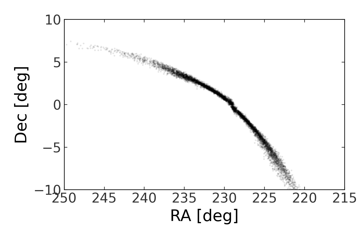Internally, this position is integrated backwards to the earliest time, then a stream is generated forward from the past time. This is particularly useful when trying to reproduce observed streams, such as the Pal 5 stream:

>>> import astropy.coordinates as coord
>>> pal5_c = coord.SkyCoord(ra=229.018*u.degree, dec=-0.124*u.degree,
...                         distance=22.9*u.kpc,
...                         pm_ra_cosdec=-2.296*u.mas/u.yr,
...                         pm_dec=-2.257*u.mas/u.yr,
...                         radial_velocity=-58.7*u.km/u.s)
>>> rep = pal5_c.transform_to(coord.Galactocentric()).data
>>> pal5_w0 = gd.PhaseSpacePosition(rep)
>>> pal5_mass = 2.5e4 * u.Msun
>>> pal5_pot = gp.PlummerPotential(m=pal5_mass, b=4*u.pc, units=galactic)
>>> mw = gp.MilkyWayPotential(version="latest")
>>> gen_pal5 = ms.MockStreamGenerator(df, mw, progenitor_potential=pal5_pot)
>>> pal5_stream, _ = gen_pal5.run(pal5_w0, pal5_mass,
...                               dt=-1 * u.Myr, n_steps=4000)
>>> pal5_stream_c = pal5_stream.to_coord_frame(coord.ICRS())

(Source code, png, pdf)

References

[fardal15] (1,2,3,4)

Fardal, Huang, Weinberg (2015)

[kuepper12]

Küpper, Lane, Heggie (2012)

[gibbons14]

Gibbons et al. (2014)

[chen24]

Chen et al. (2024)

API

Functions

mockstream_dop853(nbody, time, stream_w0, ...)

Classes

BaseStreamDF([lead, trail, random_state])	A base class for representing distribution functions for generating stellar streams.
ChenStreamDF([lead, trail, random_state])	A class for representing the Chen+2024 distribution function for generating stellar streams based on Chen et al. 2024 https://ui.adsabs.harvard.edu/abs/2024arXiv240801496C/abstract.
FardalStreamDF([gala_modified, lead, trail, ...])	A class for representing the Fardal+2015 distribution function for generating stellar streams based on Fardal et al. 2015 https://ui.adsabs.harvard.edu/abs/2015MNRAS.452..301F/abstract.
LagrangeCloudStreamDF(v_disp[, lead, trail, ...])	A class for representing the Lagrange Cloud Stripping distribution function for generating stellar streams.
MockStream(pos[, vel, frame, release_time, ...])	Represents phase-space positions, i.e. positions and conjugate momenta (velocities).
MockStreamGenerator(df, hamiltonian[, ...])	Generate a mock stellar stream in the specified external potential.
StreaklineStreamDF	A class for representing the "streakline" distribution function for generating stellar streams based on Kuepper et al. 2012 https://ui.adsabs.harvard.edu/abs/2012MNRAS.420.2700K/abstract.

Class Inheritance Diagram