Benefits of Gala
>>> import astropy.units as u
>>> import numpy as np
>>> import gala.integrate as gi
>>> import gala.dynamics as gd
>>> import gala.potential as gp
>>> from gala.units import galactic
Commonly used Galactic gravitational potentials
Create potential objects that know how to compute the gradient, energy, etc. at a given position:
>>> pot = gp.IsochronePotential(m=1E10*u.Msun, b=15.*u.kpc, units=galactic)
>>> pot.energy([8.,6.,7.]*u.kpc)
<Quantity [-0.00131002] kpc2 / Myr2>
>>> pot.gradient([8.,6.,7.]*u.kpc)
<Quantity [[1.57813742e-05],
           [1.18360306e-05],
           [1.38087024e-05]] kpc / Myr2>
Extensible and easy to define new potentials
New potentials can be easily defined by subclassing the base potential class,
PotentialBase. For faster orbit integration and computation,
you can also define potentials with functions that evaluate its derived
quantities in C by subclassing CPotentialBase. For fast
creation of potentials for quick testing, you can also create a potential
class directly from an equation that expresses the potential:
>>> SHOPotential = gp.from_equation("1/2*k*x**2", vars="x", pars="k",
...                                 name='HarmonicOscillator')
(note: this requires sympy).
Classes created this way can then be instantiated and used like any other
PotentialBase subclass:
>>> pot = SHOPotential(k=1.)
>>> pot.energy([1.])
<Quantity [0.5]>
Extremely fast orbit integration
Most of the guts of the built-in potential classes are implemented in C, enabling extremely fast orbit integration for single or composite potentials:
>>> pot = gp.IsochronePotential(m=1E10*u.Msun, b=15.*u.kpc, units=galactic)
>>> w0 = gd.PhaseSpacePosition(pos=[7.,0,0]*u.kpc,
...                            vel=[0.,50.,0]*u.km/u.s)
>>> import timeit
>>> timeit.timeit(lambda: gp.Hamiltonian(pot).integrate_orbit(w0, dt=0.5, n_steps=10000), number=100) / 100.
0.0028513244865462184
For a composite potential:
>>> bulge = gp.IsochronePotential(m=2E10*u.Msun, b=0.5*u.kpc, units=galactic)
>>> disk = gp.MiyamotoNagaiPotential(m=6E10*u.Msun, a=3*u.kpc, b=0.26*u.kpc, units=galactic)
>>> pot = gp.CCompositePotential(bulge=bulge, disk=disk)
>>> timeit.timeit(lambda: gp.Hamiltonian(pot).integrate_orbit(w0, dt=0.5, n_steps=10000), number=100) / 100.
0.0031369362445548177
Precise integrators
The default orbit integration routine uses LeapfrogIntegrator,
but the high-order Dormand-Prince 853 integration scheme is also implemented as
DOPRI853Integrator:
>>> orbit = gp.Hamiltonian(pot).integrate_orbit(w0, dt=0.5, n_steps=10000,
...                             Integrator=gi.DOPRI853Integrator)
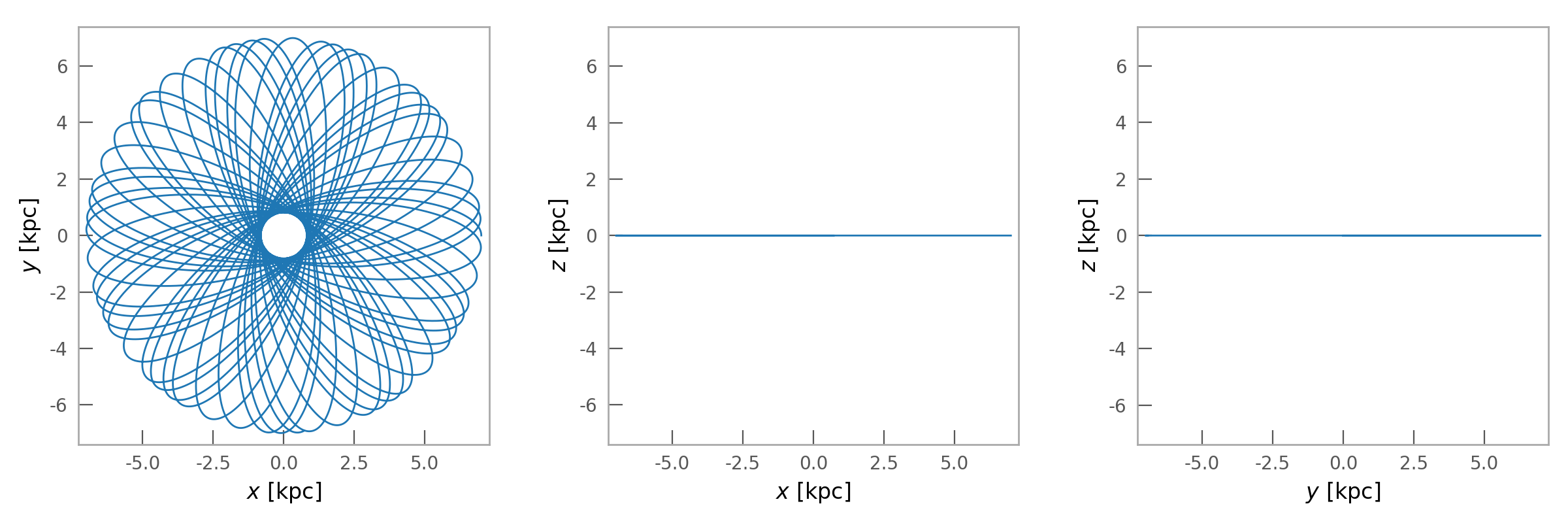
Easy visualization
Numerically integrated orbits can be easily visualized using the
plot() method:
>>> orbit.plot()
(Source code, png)

Astropy units support
All functions and classes have Astropy unit support built in: they accept and
return Quantity objects wherever possible. In addition, this
package uses an experimental new UnitSystem class for storing
systems of units and default representations.