Integrating an orbit in a rotating reference frame

We first need to import some relevant packages:

>>> import astropy.units as u
>>> import matplotlib.pyplot as plt
>>> import numpy as np
>>> import gala.integrate as gi
>>> import gala.dynamics as gd
>>> import gala.potential as gp
>>> from gala.units import galactic
>>> from scipy.optimize import minimize

Orbits in a barred galaxy potential

In the example below, we will work use the galactic UnitSystem: as I define it, this is: \({\rm kpc}\), \({\rm Myr}\), \({\rm M}_\odot\).

For this example, we’ll use a simple, analytic representation of the potential from a Galactic bar and integrate an orbit in the rotating frame of the bar, which has some pattern speed \(\Omega\). We’ll use a three-component potential model consisting of the bar (an implementation of the model used in Long & Murali 1992), a Miyamoto-Nagai potential for the galactic disk, and a spherical NFW potential for the dark matter distribution. We’ll tilt the bar with respect to the x-axis by 25 degrees (the angle alpha below). First, we’ll define the disk and halo potential components:

>>> disk = gp.MiyamotoNagaiPotential(
...     m=6e10 * u.Msun, a=3.5 * u.kpc, b=280 * u.pc, units=galactic
... )
>>> halo = gp.NFWPotential(m=6e11 * u.Msun, r_s=20.0 * u.kpc, units=galactic)

We’ll set the mass of the bar to be 1/6 the mass of the disk component, and we’ll set the long-axis scale length of the bar to \(4~{\rm kpc}\). We can now define the bar component:

>>> bar = gp.LongMuraliBarPotential(
...     m=1e10 * u.Msun,
...     a=4 * u.kpc,
...     b=0.8 * u.kpc,
...     c=0.25 * u.kpc,
...     alpha=25 * u.degree,
...     units=galactic,
... )

The full potential is the composition of the three potential objects. We can combine potential classes by defining a CCompositePotential class and adding named components:

>>> pot = gp.CCompositePotential()
>>> pot["disk"] = disk
>>> pot["halo"] = halo
>>> pot["bar"] = bar

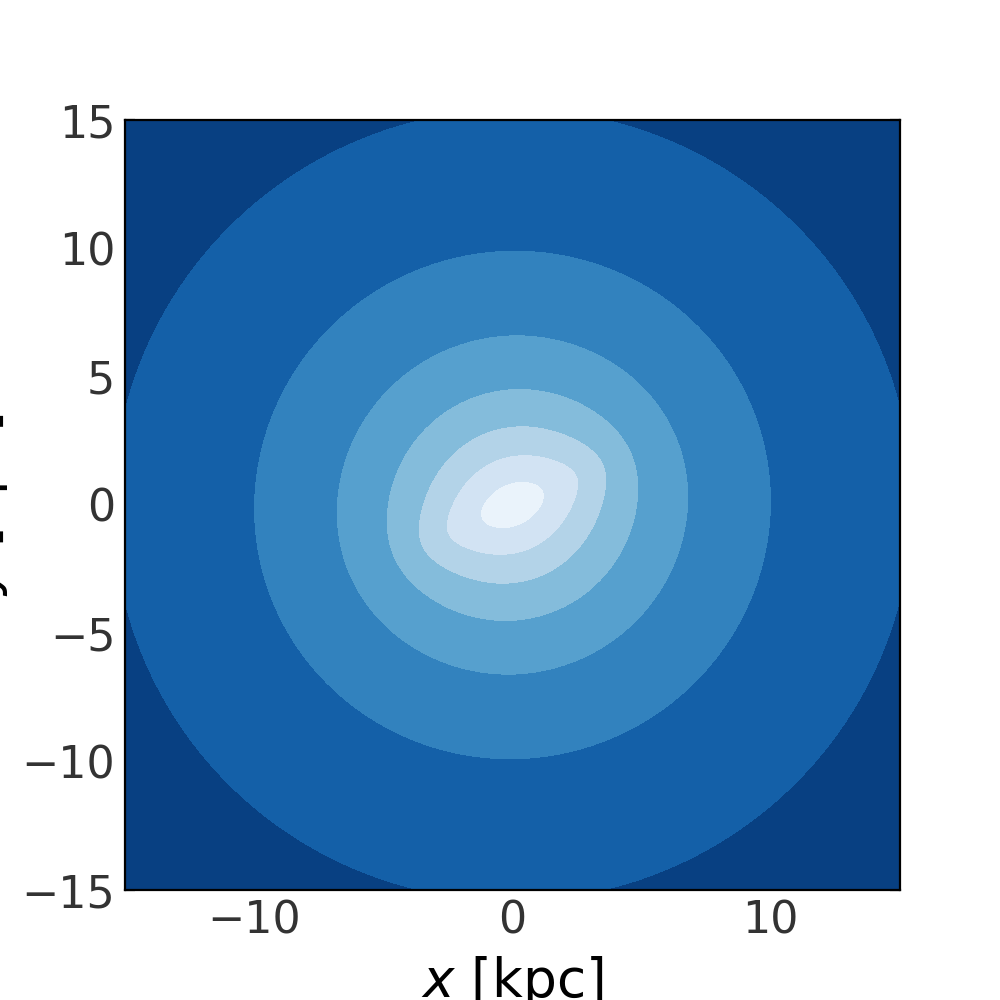
Let’s visualize the isopotential contours of the potential in the x-y plane to see the bar perturbation:

>>> grid = np.linspace(-15,15,128)
>>> fig, ax = plt.subplots(1, 1, figsize=(5,5)) 
>>> fig = pot.plot_contours(grid=(grid,grid,0.), ax=ax) 
>>> ax.set_xlabel("$x$ [kpc]") 
>>> ax.set_ylabel("$y$ [kpc]") 

(Source code, png, pdf)

We assume that the bar rotates around the z-axis so that the frequency vector is just \(\boldsymbol{\Omega} = (0,0,42)~{\rm km}~{\rm s}^{-1}~{\rm kpc}^{-1}\). We’ll create a Hamiltonian object with a ConstantRotatingFrame with this frequency:

>>> Om_bar = 42. * u.km/u.s/u.kpc
>>> frame = gp.ConstantRotatingFrame(Omega=[0,0,Om_bar.value]*Om_bar.unit,
...                                  units=galactic)
>>> H = gp.Hamiltonian(potential=pot, frame=frame)

We can now numerically find the co-rotation radius in this potential and integrate an orbit from a set of initial conditions near the co-rotation radius:

>>> import scipy.optimize as so
>>> def func(r):
...     Om = pot.circular_velocity([r[0], 0, 0] * u.kpc)[0] / (r[0] * u.kpc)
...     return (Om - Om_bar).to(Om_bar.unit).value**2
>>> res = so.minimize(func, x0=10.0, method="powell")
>>>
>>> r_corot = res.x[0] * u.kpc
>>> v_circ = Om_bar * r_corot * u.kpc
>>>
>>> w0 = gd.PhaseSpacePosition(
...     pos=[r_corot.value, 0, 0] * r_corot.unit,
...     vel=[0, v_circ.value, 0.0] * v_circ.unit,
... )
>>> orbit = H.integrate_orbit(
...     w0, dt=0.1, n_steps=40000, Integrator=gi.DOPRI853Integrator
... )
>>> fig = orbit.plot(marker=",", linestyle="none", alpha=0.5)  
>>> for ax in fig.axes: 
...     ax.set_xlim(-15,15) 
...     ax.set_ylim(-15,15) 

(Source code, png, pdf)

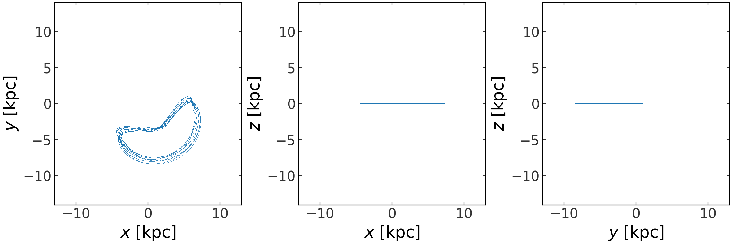
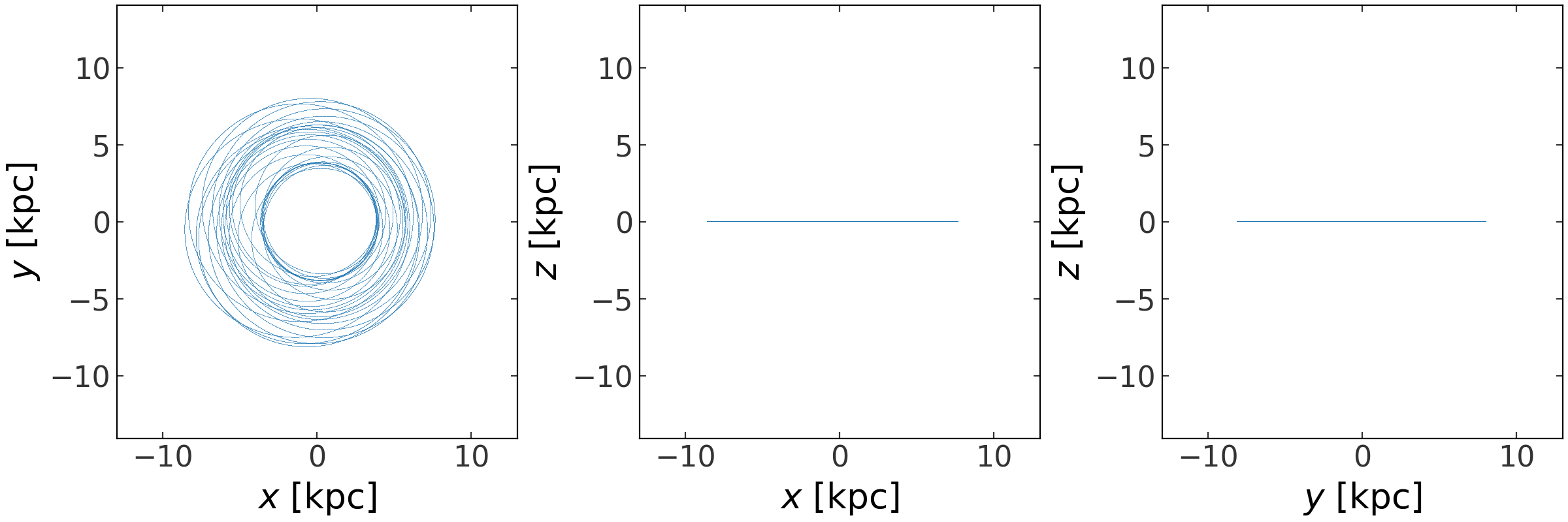
This is an orbit circulation around the Lagrange point L5! Let’s see what this orbit looks like in an inertial frame:

>>> inertial_orbit = orbit.to_frame(gp.StaticFrame(galactic))
>>> fig = inertial_orbit.plot(marker=',', linestyle='none', alpha=0.5) 
>>> for ax in fig.axes: 
...     ax.set_xlim(-15,15) 
...     ax.set_ylim(-15,15) 

(Source code, png, pdf)